
Approximating Pi
Loading the math board and drawing, please wait…
In collections
Pi Approximations
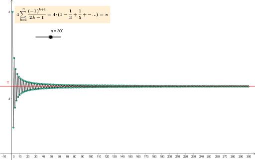
This example demonstrates the approximation of Pi by dynamically constructing polygons. It involves core mathematical concepts like limits, the circle constant Pi, and polygon area. The construction uses GeoGebra commands Sequence and PolyLine, along with objects like L, s, P for dynamic visualization. Suitable for high school mathematics education to understand the limit concept and the geometric meaning of Pi.
GeoGebra Commands & Parameters
Sequence(Sum[(4 * (-1)^(k + 1) / ((2 * k) - 1)), k, 1, j], j, 1, n) → LSequence((k, L(k)), k, 1, n) → PPolyLine(P) → f
AI Drawing Prompt Reference
Draw a dynamic polyline graph that approximates pi. The horizontal axis represents the term index, and the vertical axis represents the partial sum of the Leibniz series. First, compute the partial sums for each term count from 1 to n, where each sum is calculated by adding alternating terms of the form 4 divided by odd numbers. Then, plot points with x-coordinate equal to the term index and y-coordinate equal to the corresponding partial sum. Connect these points in order with straight line segments to form a polyline. As the term count increases, the polyline should oscillate and gradually converge to a horizontal line at the value pi divided by four. Clearly show the trend and label the axes.
The prompt above was compiled from the original drawing commands and is for reference only.