
Approximating a Definite Integral from Graph
Loading the math board and drawing, please wait…
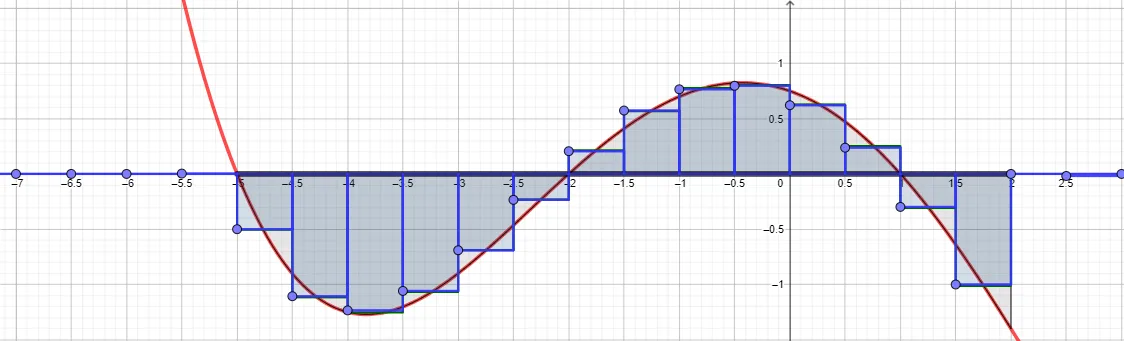
This GeoGebra template provides a dynamic visual demonstration of approximating a definite integral under a curve f(x) over an interval [a, b] using rectangular approximations (Riemann sums). The core mathematical concepts involved include the geometric interpretation of the definite integral as the net accumulated area, the concept of limits as the partition size approaches infinity, and numerical integration techniques. In terms of GeoGebra construction, the tool utilizes the Integral command to show the exact area, while Rectangle, Sequence, Point, and Segment commands are employed to generate the sequence of approximating rectangles. Interactive input boxes (associated with objects like a, b, and f) allow users to dynamically modify the integration limits, the function formula, and the number of subintervals, providing a hands-on way to observe how the sum of the rectangular areas converges to the actual integral value. This resource is highly suitable for high school and introductory college calculus students aiming to build a solid geometric intuition for integration.
GeoGebra Commands & Parameters
Textfield(f) → InputBox1Textfield(a) → InputBox2Textfield(b) → InputBox3Integral(f, a, b) → iSegment((a, 0), (b, 0)) → mSequence(Segment[(a + k / 2, 0), (a + k / 2, f(a + k / 2))], k, 0, n) → l1Sequence(Polygon[(a + (k - 1) / 2, 0), (a + (k - 1) / 2, (2 * Integral[f, a + (k - 1) / 2, a + k / 2])), (a + k / 2, (2 * Integral[f, a + (k - 1) / 2, a + k / 2])), (a + k / 2, 0)], k, 1, n) → l2Sequence(x = k / 2, k, -20, 20) → VLPoint(VL) → ARectangle(A) → q1, g, h, j, kPoint(VL) → BRectangle(B) → q2, l, p, q, rPoint(VL) → DRectangle(D) → q4, g_1, h_1, i_1, j_1Point(VL) → ERectangle(E) → q5, k_1, l_1, m_1, n_1Point(VL) → FRectangle(F) → q6, p_1, q_1, r_1, s_1Point(VL) → HRectangle(H) → q8, d_1, e_1, f_2, g_2Point(VL) → IRectangle(I) → q9, h_2, i_2, j_2, k_2Point(VL) → JRectangle(J) → q10, l_2, m_2, n_2, p_2Point(VL) → KRectangle(K) → q11, q_2, r_2, s_2, t_2Point(VL) → LRectangle(L) → q12, a_2, b_2, c_2, d_2Point(VL) → MRectangle(M) → q13, e_2, f_3, g_3, h_3Point(VL) → NRectangle(N) → q14, i_3, j_3, k_3, l_3Point(VL) → ORectangle(O) → q15, m_3, n_3, p_3, q_3Point(VL) → PRectangle(P) → q16, r_3, s_3, t_3, a_3Point(VL) → QRectangle(Q) → q17, b_3, c_3, d_3, e_3Point(VL) → SRectangle(S) → q19, j_4, k_4, l_4, m_4Point(VL) → TRectangle(T) → q20, n_4, p_4, q_4, r_4Point(VL) → VRectangle(V) → q22, c_4, d_4, e_4, f_5Point(VL) → WRectangle(W) → q23, g_5, h_5, i_5, j_5Point(VL) → ZRectangle(Z) → q24, k_5, l_5, m_5, n_5Point(VL) → A_1Rectangle(A_1) → q25, p_5, q_5, r_5, s_5Point(VL) → B_1Rectangle(B_1) → q26, t_5, a_5, b_5, c_5Point(VL) → C_1Rectangle(C_1) → q27, d_5, e_5, f_6, g_6Point(VL) → D_1Rectangle(D_1) → q28, h_6, i_6, j_6, k_6Point(VL) → E_1Rectangle(E_1) → q29, l_6, m_6, n_6, p_6Point(VL) → F_1Rectangle(F_1) → q30, q_6, r_6, s_6, t_6Point(VL) → G_1Rectangle(G_1) → q31, a_6, b_6, c_6, d_6Point(VL) → H_1Rectangle(H_1) → q32, e_6, f_7, g_7, h_7Point(VL) → I_1Rectangle(I_1) → q33, i_7, j_7, k_7, l_7Point(VL) → J_1Rectangle(J_1) → q34, m_7, n_7, p_7, q_7Point(VL) → K_1Rectangle(K_1) → q35, r_7, s_7, t_7, a_7Point(VL) → L_1Rectangle(L_1) → q36, b_7, c_7, d_7, e_7Point(VL) → M_1Rectangle(M_1) → q37, f_8, g_8, h_8, i_8Point(VL) → N_1Rectangle(N_1) → q38, j_8, k_8, l_8, m_8Point(VL) → O_1Rectangle(O_1) → q39, n_8, p_8, q_8, r_8Point(VL) → P_1Rectangle(P_1) → q40, s_8, t_8, a_8, b_8Point(VL) → Q_1Rectangle(Q_1) → q41, c_8, d_8, e_8, f_9Point(VL) → R_1Rectangle(R_1) → q42, g_9, h_9, i_9, j_9Point(VL) → GRectangle(G) → q7, t_1, a_1, b_1, c_1Point(VL) → RRectangle(R) → q18, f_4, g_4, h_4, i_4Point(VL) → V_1Rectangle(V_1) → q46, d_9, e_9, f_{10}, g_{10}
AI Drawing Prompt Reference
Create a dynamic visualization of approximating a definite integral. Show a function curve on a coordinate plane, with a series of equal-width rectangles under the curve approximating the area between the curve and the x-axis. The rectangle heights follow the function values. Mark the integration interval with a segment on the x-axis, and display the exact integral as a shaded region. Include three input boxes for adjusting the function, lower and upper limits, and the number of rectangles, plus vertical grid lines for reference. The overall effect illustrates convergence from discrete sums to the continuous area.
The prompt above was compiled from the original drawing commands and is for reference only.