
Animation 5: Trapezoid Area Variation
Loading the math board and drawing, please wait…
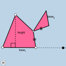
This example demonstrates the variation of trapezoid area. Key mathematical concepts include the trapezoid area formula, slope, and standard deviation. Using GeoGebra commands such as Line, Ray, Point, Segment, Slope, PointIn, Midpoint, Dilate, Rotate, Polygon, etc., the deformation process of the trapezoid can be dynamically displayed. Suitable for high school mathematics education, particularly for coordinate geometry and function graphing.
GeoGebra Commands & Parameters
Line(A, B) → fRay(A, B) → gPoint(g) → CRay(A, C) → hSegment(A, C) → iSlope(i) → mPointIn(a) → DLine(D, i) → jPoint(j) → ERay(D, E) → kPoint(k) → FSegment(D, F) → lSegment(A, D) → nSegment(F, C) → pMidpoint(p) → GDilate(A, If[0 < c ≤ 1, 1 - c, 0], C) → A'Segment(A, A') → qDilate(C, If[1 < c ≤ 2, 2 - c, 0], G) → C'Segment(C, C') → rDilate(G, If[2 < c ≤ 3, 3 - c, 0], F) → G'Segment(G, G') → sRotate(C, If[3 < c ≤ 4, ((c - 3) * π), π], G) → C'_1Rotate(C', If[3 < c ≤ 4, ((c - 3) * π), π], G) → C''Segment(C'_1, C'') → r'Dilate(F, If[4 < c ≤ 5, 5 - c, 0], D) → F'Segment(F, F') → tDilate(D, If[5 < c ≤ 6, 6 - c, 0], A) → D'Segment(D, D') → dDilate(D, If[6.5 < c ≤ 7.5, 7.5 - c, 0], G) → D'_1Polygon(A, C, G, D) → poly1, a_1, c_1, g_1, d_1Polygon(G, F, D) → poly2, d_2, g_2, f_1Segment(D, D'_1) → eRotate(G, If[8 < c ≤ 9, ((-(c - 8)) * π), π], G) → G'_1Rotate(F, If[8 < c ≤ 9, ((-(c - 8)) * π), π], G) → F'_1Rotate(D, If[8 < c ≤ 9, ((-(c - 8)) * π), π], G) → D'_2Polygon(G'_1, F'_1, D'_2) → poly2', d'_2, g'_1, f'_1Segment(F'_1, D'_2) → h_1Rotate(D, If[8 < c ≤ 9, ((-(c - 8)) * π), π], G) → D'_3Rotate(D'_1, If[8 < c ≤ 9, ((-(c - 8)) * π), π], G) → HSegment(D'_3, H) → e'Rotate(C'_1, If[8 < c ≤ 9, ((-(c - 8)) * π), π], G) → IRotate(C'', If[8 < c ≤ 9, ((-(c - 8)) * π), π], G) → C'''Segment(I, C''') → r''OrthogonalLine(D, q) → i_1Intersect(f, q) → JDilate(D, If[6 < c ≤ 7, 7 - c, 0], J) → D'_4Segment(D, D'_4) → j_1Min(t, q) → oCircle(J, (0.15 * o)) → e_1Intersect(e_1, i_1) → K, LIntersect(e_1, f) → M, NAngle(D, J, A) → αAngle(C, A, D) → βIntersect(i_1, f) → ODilate(D, If[6 < c ≤ 7, 7 - c, 0], O) → D'_5Segment(D, D'_5) → k_1Angle(A, O, D) → γPoint(f) → PPoint(f) → QCircle(C, t) → p_1Intersect(p_1, f, 2) → RRay(R, Q) → m_1Angle(F, C, A) → δ