
A Perfect Square
Loading the math board and drawing, please wait…
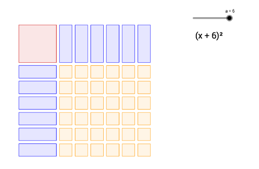
This example demonstrates the dynamic construction of a perfect square and its related properties, involving core mathematical concepts such as polygon construction, sequence application, vector operations, and intersection calculations in three-dimensional space. It utilizes GeoGebra commands like Polygon and Sequence, along with objects like a, A, B, C, D, poly1, a_1, b, d, c, text1, text2, list1, list2, list3. Suitable for high school and above learners to understand the integration of three-dimensional geometry and sequences.
GeoGebra Commands & Parameters
Polygon(A, B, D, C) → poly1, a_1, b, d, cSequence(Polygon[(3.25 + (1.25 * n), 3), (4.25 + (1.25 * n), 3), (4.25 + (1.25 * n), 0), (3.25 + (1.25 * n), 0)], n, 0, a - 1, 1) → list1Sequence(Polygon[(0, -0.25 - (1.25 * n)), (0, -1.25 - (1.25 * n)), (3, -1.25 - (1.25 * n)), (3, -0.25 - (1.25 * n))], n, 0, a - 1, 1) → list2Sequence(Sequence[Polygon[(3.25 + (1.25 * n), -0.25 - (1.25 * m)), (4.25 + (1.25 * n), -0.25 - (1.25 * m)), (4.25 + (1.25 * n), -1.25 - (1.25 * m)), (3.25 + (1.25 * n), -1.25 - (1.25 * m))], n, 0, a - 1, 1], m, 0, a - 1, 1) → list3