
Standard Deviation and Distribution Visualization by David Wees (3)
Loading the math board and drawing, please wait…
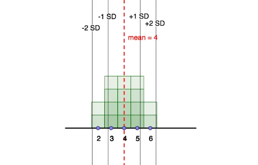
This example visually demonstrates the concepts of standard deviation and distribution. It involves core statistical concepts such as data distribution, mean, median, and mode. Using GeoGebra commands like Segment, Point, Line, Frequency, Mode, Sequence, SD, users can dynamically observe changes in data distribution. Suitable for high school and above students or teachers for teaching and learning probability and statistics.
GeoGebra Commands & Parameters
Segment((0, 0), (9, 0)) → gPoint(g) → MPoint(g) → QPoint(g) → NPoint(g) → LPoint(g) → KPoint(g) → PPoint(g) → CPoint(g) → DPoint(g) → EPoint(g) → FPoint(g) → GPoint(g) → HPoint(g) → IPoint(g) → JPoint(g) → RPoint(g) → OLine(A, B) → fFrequency(list4, list1) → list5Segment((-0.5, 0), (9.5, 0)) → iMode(list1) → list3Mode(list1) → list6Sequence(Sequence[Polygon[(n - 0.5, 0), (n - 0.5, k), (n + 0.5, k), (n + 0.5, 0)], k, 1, Element[list5, n + 1], 1], n, 0, 9, 1) → list2SD(list1) → bPoint(h) → S
AI Drawing Prompt Reference
Create a visualization of standard deviation and distribution. First, draw a horizontal line segment, then place 10 points on the segment to represent data points. Next, draw a line through the first two points to indicate the central tendency of the data distribution. Use these points and lines to dynamically show data distribution, mean, median, and mode. Finally, create a frequency histogram based on the data points and calculate the standard deviation.
The prompt above was compiled from the original drawing commands and is for reference only.