
Standard Deviation and Distribution Visualization by David Wees (2)
Loading the math board and drawing, please wait…
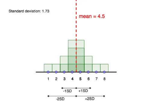
This example visualizes standard deviation and distribution. It involves core concepts in probability and statistics, using GeoGebra commands such as Segment, Point, Line, Frequency, etc., to illustrate how data distribution can be understood through standard deviation. Suitable for high school and above students or teachers to better understand the basic principles of probability and statistics.
GeoGebra Commands & Parameters
Segment((0, 0), (9, 0)) → gPoint(g) → MPoint(g) → QPoint(g) → NPoint(g) → LPoint(g) → KPoint(g) → PPoint(g) → CPoint(g) → DPoint(g) → EPoint(g) → FPoint(g) → GPoint(g) → HPoint(g) → IPoint(g) → JPoint(g) → RPoint(g) → OLine(A, B) → fFrequency(list4, list1) → list5Segment((-0.5, 0), (9.5, 0)) → iMode(list1) → list3Mode(list1) → list6Sequence(Sequence[Polygon[(n - 0.5, 0), (n - 0.5, k), (n + 0.5, k), (n + 0.5, 0)], k, 1, Element[list5, n + 1], 1], n, 0, 9, 1) → list2SD(list1) → bPoint(h) → SIntersect(h, i) → TPoint(h) → ULine(V, W) → pIntersect(l, p) → A_1Intersect(j, p) → B_1Intersect(h, p) → D_1Segment(D_1, B_1) → qSegment(D_1, A_1) → rIntersect(m, s) → ZIntersect(h, s) → C_1Intersect(k, s) → E_1Segment(C_1, Z) → tSegment(C_1, E_1) → aRay(T, U) → n