3D Vector Field Dynamic Visualization

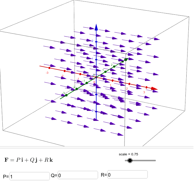
This example demonstrates how to visualize a three-dimensional vector field by allowing users to input component functions for x, y, and z directions, then rendering arrows on a grid to show direction and magnitude at each point. Core mathematical concepts include vector fields, 3D coordinate geometry, parametric functions, and the geometric interpretation of vector fields in differential equations. Construction highlights: using GeoGebra's Sequence command to generate grid points with adjustable spacing, Textfield and InputBox controls for entering component expressions, a scale parameter to control arrow length, and the vectors object for dynamic rendering. Suitable for high school to university-level mathematics education, particularly for multivariable calculus, vector analysis, or physics demonstrations of electric and magnetic fields, as well as exploring various field configurations.