
3D Matrix Transformations
Loading the math board and drawing, please wait…
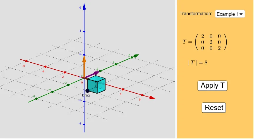
This example demonstrates the effects of matrix transformations on 3D objects like cubes and pyramids in space. Key math concepts include matrix application, transformation, vectors, and solid geometry. GeoGebra commands such as SelectedIndex, Element, Vector, Circle, Line, Intersect, Segment, Point, Cube, ApplyMatrix, Polygon, Determinant, and Sequence are used to construct the transformations, with slider animations to visualize the changes. Suitable for high school and above students to learn about matrix transformations in solid geometry.
GeoGebra Commands & Parameters
SelectedIndex(Examples) → indexElement(MT, index) → T_0Vector((0, 0, 0), (x_0, y_0, z_0)) → uVector((0, 0, 0), (x_1, y_1, z_1)) → vVector((0, 0, 0), (x_2, y_2, z_2)) → wCircle(A, 1, xOyPlane) → cLine(A, xAxis) → fIntersect(f, c, 1) → BSegment(A, B) → gPoint(Circle[B, Distance[A, B], Segment[A, B]]) → CCube(A, B, C) → Cube, D, faceCDHG, faceEFGH, edgeAD, edgeAB, edgeBC, edgeCD, edgeAE, edgeDH, edgeEH, edgeEF, E, edgeBF, edgeFG, edgeCG, edgeGH, F, G, H, faceABCD, faceADHE, faceABFE, faceBCGFApplyMatrix(T_a, A) → A'ApplyMatrix(T_a, B) → B'ApplyMatrix(T_a, C) → C'ApplyMatrix(T_a, D) → D'ApplyMatrix(T_a, E) → E'ApplyMatrix(T_a, F) → F'ApplyMatrix(T_a, G) → G'ApplyMatrix(T_a, H) → H'Polygon(A', B', C', D') → poly1, a', b', c', d'Polygon(E', A', B', F') → poly2, e', a'_1, b'_1, f'Polygon(B', C', G', F') → poly3, b'_2, c'_1, g', f'_1Polygon(A', E', H', D') → poly4, a'_2, e'_1, h', d'_1Polygon(H', D', C', G') → poly5, h'_1, d'_2, c'_2, g'_1Polygon(H', E', F', G') → poly6, h'_2, e'_2, f'_2, g'_2Determinant(T_0) → deterSequence(Sequence[Sequence[(i, j, k), i, -4, 4, 8 / 3], j, -4, 4, 8 / 3], k, -4, 4, 8 / 3) → points3dElement(points3d, 1, 1) → KKASequence(OrthogonalLine[Element[KKA, i], z = 0], i, 1, 4) → list1Element(points3d, 1, 2) → KKA1Element(points3d, 1, 3) → KKA2Element(points3d, 1, 4) → KKA3Sequence(OrthogonalLine[Element[KKA1, i], z = 0], i, 1, 4) → list2Sequence(OrthogonalLine[Element[KKA2, i], z = 0], i, 1, 4) → list3Sequence(OrthogonalLine[Element[KKA3, i], z = 0], i, 1, 4) → list4Element(points3d, 2, 1) → KAElement(points3d, 3, 1) → KA1Element(points3d, 4, 1) → KA2Sequence(OrthogonalLine[Element[KKA, i], y = 0, space], i, 1, 4) → list5Sequence(OrthogonalLine[Element[KA1, i], y = 0, space], i, 1, 4) → list6Sequence(OrthogonalLine[Element[KA, i], y = 0, space], i, 1, 4) → list7Sequence(OrthogonalLine[Element[KA2, i], y = 0, space], i, 1, 4) → list8ApplyMatrix(T_a, list1) → list1'ApplyMatrix(T_a, list2) → list2'ApplyMatrix(T_a, list3) → list3'ApplyMatrix(T_a, list4) → list4'ApplyMatrix(T_a, list5) → list5'ApplyMatrix(T_a, list6) → list6'ApplyMatrix(T_a, list7) → list7'ApplyMatrix(T_a, list8) → list8'
AI Drawing Prompt Reference
Draw a 3D cube and its image after matrix transformation in space. First, create three vectors u, v, and w, then construct a circle c and a line f based on these points. Find the intersection point B of line f and circle c, connect point A and B to form segment g, and then find the point C on circle c closest to A. Use points A, B, and C to construct the cube. Apply matrix transformation T_a to each vertex of the cube to generate a new cube and its faces and edges. Finally, generate a series of points and draw their orthogonal lines on the x-axis and y-axis, and apply the same matrix transformation T_a to these lines.
The prompt above was compiled from the original drawing commands and is for reference only.