
3D Cosine Function Modeling with Rotation
Loading the math board and drawing, please wait…
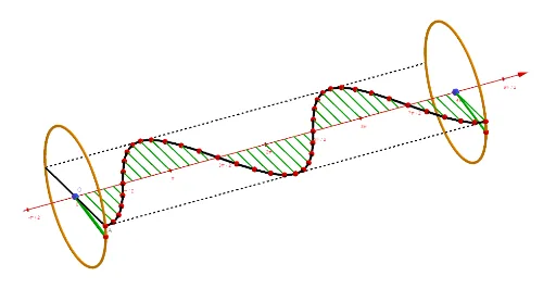
This example visualizes how the cosine function in 3D can be interpreted via geometry, linking cosine to a projection ratio as a parameter (angle) changes. It demonstrates the relationship between trigonometry, distances in right triangles (in the spirit of Pythagoras), and spatial construction using 3D transformations. The model builds a reference configuration using Circle and CircumcircleArc, then parameterizes motion with Sequence and a parameter such as t/Step, computes key points via Midpoint, and lifts the structure into 3D through Rotate and Translate. Line segments (Segment) define the geometric connectors used to read off cosine-related lengths, while CurveCartesian generates the resulting space curve/graph as the configuration evolves. Suitable for advanced middle school through early university audiences learning trigonometry with solid-geometry visualization.
GeoGebra Commands & Parameters
Circle(O, R, xAxis) → cRotate(A, (-t), xAxis) → A'Segment(O, A') → fTranslate(c, Vector[O, B]) → c'Segment(C, O') → gSegment(D, O') → hSequence((i, ((-R) * cos(i)), 0), i, 0, t, (2 * π / Step)) → l1Sequence((i, 0, 0), i, 0, t, (2 * π / Step)) → l2Sequence(Segment[Element[l1, i], Element[l2, i]], i, 1, Length[l1]) → l3Segment(O, E) → iSegment(A', E) → kSegment(E, O) → lMidpoint(O, A) → FMidpoint(O, F) → GMidpoint(A', O) → HMidpoint(H, O) → IRotate(G, ((-t)) / 2, xAxis) → G'CircumcircleArc(G, G', I) → eSegment(O, A) → mRotate(G, t / 2, xAxis) → G'_1CircumcircleArc(G, G'_1, I) → pSegment(D, C) → n_1CurveCartesian(i, R, 0, i, 0, t) → bCurveCartesian(i, (-R), 0, i, 0, t) → dSegment(O - (0, R, 0), O + (0, R, 0)) → jCurveCartesian(i, ((-R) * cos(i)), 0, i, 0, t) → aSequence(Rotate[Element[l3, i], (-(ang°)), xAxis], i, 1, Length[l1]) → l4Rotate(a, (-(ang°)), xAxis) → a'Sequence(Rotate[Element[l1, i], (-(ang°)), xAxis], i, 1, Length[l1]) → l5Rotate(j, (-(ang°)), xAxis) → j'Rotate(b, (-(ang°)), xAxis) → b'Rotate(d, (-(ang°)), xAxis) → d'
AI Drawing Prompt Reference
This is a 3D cosine function model that visualizes the relationship between cosine and angle through geometric transformations. The model uses circles and arcs to establish a reference structure, line segments connect key points, and rotations and translations elevate the structure to three dimensions. Curves generate space curves to show the shape of the cosine function as the angle changes. This model helps learners understand the connection between trigonometry and spatial geometry.
The prompt above was compiled from the original drawing commands and is for reference only.