
3D Basketball Shot and Rebound Trajectory Simulation
Loading the math board and drawing, please wait…
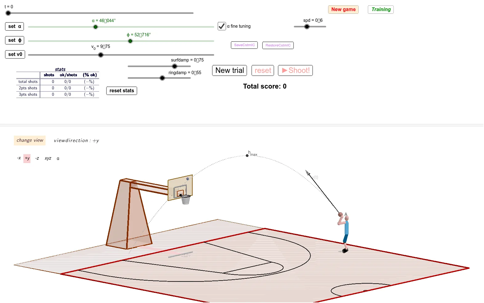
This GeoGebra example models a basketball shot in 3D, showing the ball’s projectile path, rebound behavior, and spatial relationships among the ball, hand, floor, and target. It uses vectors, initial velocity components v0_x, v0_y, v0_z, gravity g, ball radius rball, planes, spheres, circles, distances, intersections, closest points, rotations, translations, and locus/parametric ideas. The construction combines Point, Vector, Sphere, Plane, Circle, Segment, Distance, Intersect, ClosestPoint, Rotate, Translate, Locus, Surface, Prism, If, Min, Textfield, and TableText to define geometry, test rebound conditions, and display parameters. It is suitable for high school or introductory college courses in physics, vector geometry, coordinate geometry, and dynamic modeling.
GeoGebra Commands & Parameters
Min(sqrt(x(G12toeR)^(2) + y(G12toeR)^(2)), sqrt(x(G12toeL)^(2) + y(G12toeL)^(2))) → GtoedistSegment(Ghand_L0, G4_L) → gghandsho_L0Distance(GHLdet, G4_L) → GHLradIntersect(yAxis, xAxis) → OMirror(E_1, O) → E_2Semicircle(E_1, E_2) → cDistance(A_{xy}, O) → distAIf(t < t_c, ωk, (ℯ^((-(t - t_c))) * ωk)) → ωDistance(Hxy2, C_c) → dist2_{ring}Distance(Hxy1, C_c) → dist1_{ring}Distance(A_{xy}, (x(Vpar), y(Vpar))) → VAxyDistance(GHRdet, G4_R) → GHRradIf(t < td, Point[{GHLx(t), GHLy(t), GHLz(t)}], Point[{GHLx2(t), GHLy2(t), GHLz2(t)}]) → Ghand_LIf(sqrt((x(G4_L) - x(O'))^(2) + (y(G4_L) - y(O'))^(2)) - sqrt((x(Ghand_L) - x(O'))^(2) + (y(Ghand_L) - y(O'))^(2)) > 0, 1, -1) → fwd_LVector(((((-fwd_L) * cos(α)) * cos(π / 2 - ϕhs_{LR})), (((-fwd_L) * sin(α)) * cos(π / 2 - ϕhs_{LR})), ((-fwd_L) * cos(ϕhs_{LR})))) → elbdisp_{unitLR}Distance(Ghand_L, G4_L) → gghandsho_LIf(gghandsho_L^(2) > armlen^(2), 0, (1 / 2 * sqrt(armlen^(2) - gghandsho_L^(2)))) → elbdisp_LMidpoint(Ghand_L, G4_L) → elbL_0If(t < td, Point[{GHRx(t), GHRy(t), GHRz(t)}], Point[{GHRx2(t), GHRy2(t), GHRz2(t)}]) → Ghand_RDistance(Ghand_R, G4_R) → gghandsho_RMirror(U_1, Xf) → U_2Mirror(U_3, Xc) → U_4Segment(E_1, U_1) → u_1Segment(E_2, U_2) → u_2Mirror(U_5, Xf) → U_6Mirror(U_7, Xc) → U_8Polygon(U_5, U_3, U_4, U_6) → poly1, u_5, u_3, u_4, u_6Semicircle(U_8, U_7) → dSurface(((R_{ring} + (r_{ring} * cos(u))) * cos(v)), ((R_{ring} + (r_{ring} * cos(u))) * sin(v)), (r_{ring} * sin(u)) + h, u, 0, (2 * π), v, 0, (2 * π)) → ringPolygon(T_1, T_2, T_4, T_3) → poly_{bckb}, t_1, t_2, t_4, t_3Segment(C_b, C_t) → csostDilate(poly_{bckb}, 0.5, C_t) → poly2_{tabint}Dilate(poly_{bckb}, 0.25, C_t) → poly2_{sost}Prism(poly2_{sost}, -3.1998318771914116) → a, B, edge1, edge2, edge3, edge4, edge5, edge6, edge7, edge8, C, D, E, face1, face2, face3, face4, face5Mirror(U_9, Xff) → U_{10}Polygon(U_5, U_9, U_{10}, U_6) → poly2, u_7, u_9, u_{10}, u_8Polygon(C, C', C_{xyr}, C_{xy}) → poly3, c_1, c', c_{xyr}, c_{xy}Polygon(B, B', B_{xyr}, B_{xy}) → poly4, b, b', b_{xyr}, b_{xy}Polygon(B', C', C, B) → poly5, b'_1, c'_1, c_2, b_1Polygon(B_{xyr}, C_{xyr}, C', B') → poly6, b_2, c_3, c'_2, b'_2Polygon(C_{xy}, B_{xy}, B, C) → poly7, c_4, b_3, b_4, c_5Point(face2) → GSegment(F, G) → fMirror(F, planexz) → F'Mirror(G, planexz) → G'Segment(F', G') → f'CurveCartesian(((-u)) / 5 + R_{ring}, 0, h - u, u, 0, 0.4) → fnetSurface(fnet, 360°, zAxis) → netVector(A, A') → uSegment(A, A_{xy}) → iMirror(TL1, Xf) → TL1'Mirror(TL2, xAxis) → TL2'Semicircle(TL2, TL2') → kSegment(TL1, TL2) → jSegment(TL1', TL2') → lSegment(TL2', TL2) → mCurveCartesian((x(P) - (w * cos(α)), y(P) - (w * sin(α)), z(P) + (w * (((-g) * t) + v0_z) / v0_s)), w, -2 / v_0, 4 / v_0) → tgtraIf(resultptsnew ≟ 3, "OK - 3pts", resultptsnew ≟ 2, "OK - 2pts", "Fail") → resultCurveCartesian(((v0_x * t) + x(A), (v0_y * t) + y(A), ((-1 / 2 * g) * t^(2)) + (v0_z * t) + z(A)), t, 0, tz_0) → traIf((checkv0 < 0) ∧ (checkv0_m > 0), (v_0 / g * sqrt(v_0^(2) - ((2 * g) * (h - z(A))))), distA) → s0_{cond}Segment(G4, G0) → trunkSegment(G6, G8) → legl_2Segment(G0, G6) → legl_1Segment(G0, G7) → legr_1Segment(G7, G9) → legr_2Line(A_{xy}, O) → nOrthogonalLine(A_{xy}, n, xOyPlane) → pLine(G1, p) → qRotate(Head, headangle, q) → Head'Segment(G9, G12toeL) → footLSegment(G8, G12toeR) → footRMidpoint(Ghand_R, G4_R) → elbR_0Translate(elbL_0, Vector[(elbdisp_L * elbdisp_{unitLR})]) → Gelb_LSegment(Gelb_L, Ghand_L) → arml_2Segment(G4_L, Gelb_L) → arml_1If(gghandsho_R^(2) > armlen^(2), 0, (1 / 2 * sqrt(armlen^(2) - gghandsho_R^(2)))) → elbdisp_RTranslate(elbR_0, Vector[(elbdisp_R * elbdisp_{unitLR})]) → Gelb_RSegment(Gelb_R, Ghand_R) → armr_2Segment(G4_R, Gelb_R) → armr_1If(gghandsho_R > armlen, false, t) → oDistance(Ghand_L0, (x(A) + (rball * cos(α - π / 4)) + (v0_x * t), y(A) + (rball * sin(α - π / 4)) + (v0_y * t), z(A) - (rball * sin(ϕ)) - ((1 / 2 * g) * t^(2)) + (v0_z * t))) → distxLine(elbL_0, elbdisp_{unitLR}) → elbline_LLine(elbR_0, elbdisp_{unitLR}) → elbline_RLocus(Ghand_L, t) → loc1Textfield(timelimit) → SetGameTimeIf(condtot, If[Gtoedist > 6.25, 3, 2], 0) → eIf(0 < t < t_c, true, false) → flyingballIf(time - floor(time) ≥ 0.95, LaTeX[floor(time + 1) + ".0"], If[time - floor(time) < 0.05, LaTeX[floor(time) + ".0"], LaTeX[round(time, 1)]]) → timeroundfix1TableText({{"", "shots", "ok/shots", "ok%"}, {"total shots", 2, 3, 4}, {"2pts shots", 2, 3, 4}, {"3pts shots", 2, 3, 4}, {1, 2, 3, 4}}, "c_|||h") → ttxtestPolygon(U_3, U_4, U_{10}, U_9) → polyfloor, r, s, f_1, g_1Circle(O_{ring}, R_{ring}, zAxis) → liringVector(A, A + Dilate[ic00(2), vsca]) → uvSphere(Prun, rball) → ball_1If(Distance[Prun, liring] < r_{ring} + rball, true, false) → impringClosestPoint(liring, Prun) → QLine(Prun, Q) → pqIf(Distance[Prun, plaz] < rball + 0.02, true, false) → impfloorIf(Distance[Prun, ClosestPointRegion[poly_{bckb}, Prun]] < rball, true, false) → impbackboardPlane(A, AV, Vpar) → αplaCircle((x(Prun), y(Prun), 0), rball, xOyPlane) → ballshdwSegment((x(T_3), y(T_3), 0), (x(T_4), y(T_4), 0)) → shdwbbCircle((x(O_{ring}), y(O_{ring}), 0), R_{ring}, zAxis) → ringshdwElement(listvectordirection, If[faces > 0, faces, 5]) → SelectedvectorSegment((x(C_t), y(C_t), 0), (x(C_b), y(C_b), 0)) → shdwringsupSegment((x(G), y(G), 0), (x(D) + 0.37, y(D), 0)) → shdwGDSegment((x(G'), y(G'), 0), (x(E) + 0.37, y(E), 0)) → shdwG'EPolygon((x(G), y(G), 0.02), (x(G'), y(G'), 0.02), (x(E) + 0.42, y(E), 0.02), (x(D) + 0.42, y(D), 0.02)) → shdwsup, h_1, i_1, j_1, k_1Dilate(d, 0.1, Xc) → d_cCurveCartesian(((x(ic(2)) * τ) + x(ic(1)), (y(ic(2)) * τ) + y(ic(1)), ((-1 / 2 * g) * τ^(2)) + (z(ic(2)) * τ) + z(ic(1))), τ, 0, tzrun_0) → trarunDilate(vvar, vsca) → vvar'Translate(Prun, Vector[Dilate[vvar', 0.95]]) → vtpointIf(tresultpts, If[Gtoedist ≥ 6.25, 3, 2], 0) → resultptsIf((z(Prun) > h - rball) ∧ (z(Prun) < h) ∧ (z(vvar) < 0), true, false) → tresultIf(tresult_t > 0, 0, 0) → tscoreIf(x(A) ≥ 0, ((atan(y(A) / x(A)) * 180 / π))°, If[y(A) > 0, ((atan(y(A) / x(A)) * 180 / π) + 180)°, ((atan(y(A) / x(A)) * 180 / π) - 180)°]) → αtgtSegment(P, Q) → pqsegIf(αFT, αtgt - 15°, -180°) → αminFTIf(αFT, αtgt + 15°, 180°) → αmaxFT
AI Drawing Prompt Reference
A 3D basketball shot simulation showing the projectile path of the ball, basket rebound behavior, and spatial relationships among the ball, hand, floor, and target. The figure includes elements such as the ball, basket, trajectory, shooter, floor plane, and target point, combining physics motion with geometric construction.
The prompt above was compiled from the original drawing commands and is for reference only.