
3×3 Matrix Transformation 2.2 Example 1: Linear Mapping in 3D
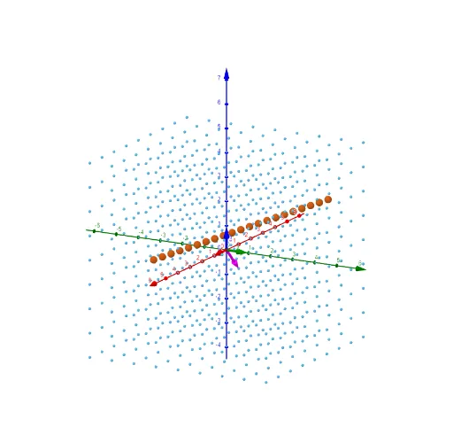
Loading the math board and drawing, please wait…
This example illustrates the geometric effect of a 3×3 matrix transformation on points, vectors, and curves in three-dimensional space, using GeoGebra's 3D graphics to compare original and transformed objects. The core mathematical concepts involve matrix multiplication, linear transformations, basis vectors (e₁, e₂, e₃), orthogonal planes, and parametric curves under transformation. The construction employs the ApplyMatrix command to transform points, vectors, and curves; OrthogonalPlane to construct orthogonal planes; Sequence to generate ordered lists; and CurveCartesian to define parametric curves. Key objects include matrix T, identity matrix I, point A, matrix M, basis vectors e₁/e₂/e₃, parameters t₁/t₂/t₃, lines d/e/f, point b, transformed points m1 and m1', lines l1 and l1', curve c, lines l2 and l2', vector u and its transformed counterpart u'. This resource is ideal for university-level linear algebra or engineering mathematics courses, and also serves as a visual aid for advanced high school students or educators to grasp the abstract nature of matrix transformations.
GeoGebra Commands & Parameters
ApplyMatrix(M, e_{1}) → t_{1}ApplyMatrix(M, e_{2}) → t_{2}ApplyMatrix(M, e_{3}) → t_{3}OrthogonalPlane((0, 0, 0), Vector[t_{1} ⊗ t_{2}]) → dOrthogonalPlane((0, 0, 0), Vector[t_{1} ⊗ t_{3}]) → eOrthogonalPlane((0, 0, 0), Vector[t_{2} ⊗ t_{3}]) → fSequence(Sequence[(2 - (2 * w) + t, w, t), w, -4, 4, 1], t, -4, 4, 1) → m1ApplyMatrix(M, m1) → m1'Sequence(Sequence[Sequence[(x_{1}, x_{2}, x_{3}), x_{1}, -4, 4, 1], x_{2}, -4, 4, 1], x_{3}, -4, 4, 1) → l1CurveCartesian((9 * t) - 3, t - 1, t, t, -5, 5) → cApplyMatrix(M, l1) → l1'Sequence(c(w), w, -1, 1, 0.1) → l2ApplyMatrix(M, l2) → l2'ApplyMatrix(M, u) → u'
AI Drawing Prompt Reference
In three-dimensional space, show the effect of a 3×3 matrix transformation. Include the origin and basis vectors e₁, e₂, e₃, along with their transformed results t₁, t₂, t₃. Construct three mutually perpendicular planes d, e, f. Then draw a sequence m1 with points (2-2w+t, w, t) where w and t range from -4 to 4. Apply the transformation to get m1'. Next, draw a parametric curve c defined for t from -5 to 5 with coordinates (9t-3, t-1, t). Apply the transformation to get l1'. Finally, show the transformed vector u and its transformed version u'. The entire figure illustrates the geometric changes through matrix transformation.
The prompt above was compiled from the original drawing commands and is for reference only.