
2D Elastic Collision Simulation of Two Hard Spheres
Loading the math board and drawing, please wait…
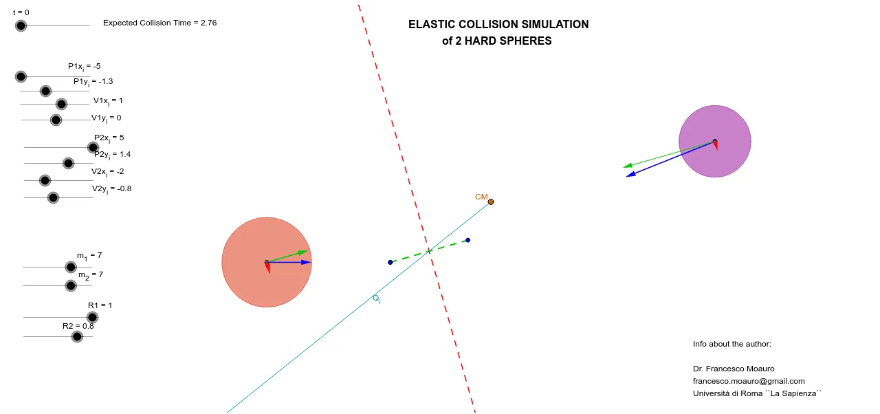
① This applet demonstrates the complete dynamic process of an elastic collision between two hard spheres in a plane, visualizing changes in velocity and position before and after impact, along with conservation of momentum and kinetic energy. ② Core mathematical concepts include conservation of momentum and kinetic energy in classical mechanics, collision geometry (normal and tangential decomposition), vector operations, and parametric equations describing motion. ③ Construction highlights: Based on the construction summary, GeoGebra commands such as Vector, Segment, LineBisector, Intersect, Rotate, Defined, and If are used to build collision points, normal vectors, velocity decomposition (parallel and perpendicular components), and post-collision velocity updates (e.g., P1para_f, P2orto_f). ④ Suitable for high school physics or introductory university physics demonstrations of collisions, as well as mathematics examples of vector decomposition and parametric equations, helping students grasp the geometric and algebraic essence of elastic collisions.
GeoGebra Commands & Parameters
Vector((0, 0), Point[{(x(P2_{urto}) - x(P1_{urto})) / NV, (y(P2_{urto}) - y(P1_{urto})) / NV}]) → V_{para}Vector((0, 0), Point[{(-(y(P2_{urto}) - y(P1_{urto}))) / NV, (x(P2_{urto}) - x(P1_{urto})) / NV}]) → V_{orto}Vector(P1_i, P1_i + (V1x_i, V1y_i)) → V1_iVector(P2_i, P2_i + (V2x_i, V2y_i)) → V2_iVector(P2_i, P2_i + P2orto_i) → V2orto_iVector(P2_i, P2_i + P2para_i) → V2para_iVector(P1_i, P1_i + P1para_i) → V1para_iVector(P2_f, P2_f + P2para_f) → V2para_fVector(P1_i, P1_i + P1orto_i) → V1orto_iSegment(P1_{urto}, P2_{urto}) → Asse_{urto}LineBisector(Asse_{urto}) → aIntersect(a, Asse_{urto}) → ARotate(P1_{urto}, 90*°, P1_{urto}) → BVector(P1_f, P1_f + (V1x_f, V1y_f)) → V1_fVector(P2_f, P2_f + (V2x_f, V2y_f)) → V2_fVector(CM, CM + PQ_f) → Q_{f}Vector(CM, CM + PQ_i) → Q_{i}Vector(P1_f, P1_f + P1para_f) → V1para_fVector(P1_f, P1_f + P1orto_f) → V1orto_fVector(P2_f, P2_f + P2orto_f) → V2orto_fDefined(t_{urto}) → AAAIf(Defined[t_{urto}], If[t < t_{urto}, Circle[P2_i, R2], Circle[P2_f, R2]], Circle[(P2x_i + V2x_i * t, P2y_i + V2y_i * t), R2]) → Palla2If(Defined[t_{urto}], If[t < t_{urto}, Circle[P1_i, R1], Circle[P1_f, R1]], Circle[(P1x_i + V1x_i * t, P1y_i + V1y_i * t), R1]) → Palla1
AI Drawing Prompt Reference
Create a 2D elastic collision simulation of two hard spheres. Show the initial positions and velocity vectors of both spheres, then the moment of contact with the normal and tangential directions at the collision point. Decompose each velocity into components parallel and perpendicular to the normal, displaying them as separate vectors. After collision, update the velocity vectors and show the new motion directions. Include sliders to control time and observe the dynamic process before and after impact. Also display the center of mass and total momentum vector to illustrate conservation laws.
The prompt above was compiled from the original drawing commands and is for reference only.