
Logistic Map Cobweb Plot and Liapunov Exponent
Loading the math board and drawing, please wait…
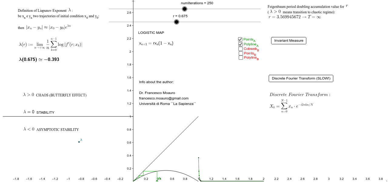
This example demonstrates the cobweb plot of the logistic map and the calculation and visualization of its Liapunov exponent, involving core mathematical concepts like the logistic map, iterative sequences, Liapunov exponent, and Fourier transform. It uses commands like Point, IterationList, Segment, Sequence, PolyLine, and objects such as numIterations, N, r, f, values, λ. Suitable for high school and above mathematics learners to understand chaos theory and dynamical systems.
GeoGebra Commands & Parameters
Point(xAxis) → AIterationList(f, x(A), numIterations) → valuesPoint(xAxis) → BSegment(A, (x(A), f(x(A)))) → bSequence(Segment[(Element[values, i], Element[values, i + 1]), (Element[values, i + 1], Element[values, i + 1])], i, 1, numIterations - 1) → cobwebHorizontalSequence(Segment[(Element[values, i], Element[values, i]), (Element[values, i], Element[values, i + 1])], i, 2, numIterations) → cobwebVerticalIterationList(f, x(B), numIterations) → valuesBSegment(B, (x(B), f(x(B)))) → cSequence(Segment[(Element[valuesB, i], Element[valuesB, i + 1]), (Element[valuesB, i + 1], Element[valuesB, i + 1])], i, 1, numIterations - 1) → cobwebHorizontalBSequence(Segment[(Element[valuesB, i], Element[valuesB, i]), (Element[valuesB, i], Element[valuesB, i + 1])], i, 2, numIterations) → cobwebVerticalBSequence((1 + i / numIterations, Element[values, i]), i, 1, numIterations) → SERIEverdeSequence((1 + i / numIterations, Element[valuesB, i]), i, 1, numIterations) → SERIErossaPolyLine(SERIEverde) → verdePolyLine(SERIErossa) → rossaPoint({-1 + r / 4, Liap + 1}) → λPoint({0, r}) → f1Point({0.5, 0}) → f2Point({1, r}) → f3PolyLine(f1, f2, f3) → assDERIVATASegment((0, 0), (1, 1)) → mSegment((-2, 1), (0, 1)) → dSequence(i / Barre, i, 0, Barre) → CLASSBOUND
AI Drawing Prompt Reference
Create a cobweb plot for the Logistic Map, showing the trajectory of iterative sequences with different colored lines for forward and reverse iterations. Calculate and visualize the Liapunov exponent, marking key points and plotting the derivative function along with a diagonal line. Finally, represent a probability distribution with bar charts in different colors.
The prompt above was compiled from the original drawing commands and is for reference only.