
旋转体与体积可视化
几何画板及绘图内容加载中,请稍等……
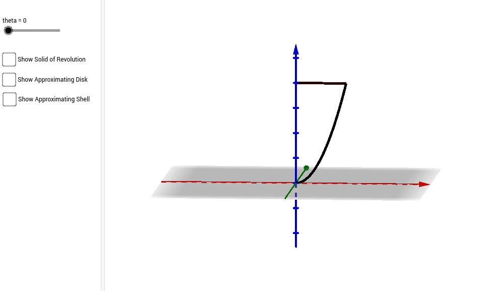
这个GeoGebra范例演示了由曲线y=x^2、x轴和y轴围成的区域绕x轴旋转生成的旋转体。涉及的核心数学概念包括函数、立体几何和微积分。通过使用CurveCartesian、Surface、Polygon等命令,可以构造旋转体的图像。适合高中数学教学和学习。
GeoGebra 命令及参数
CurveCartesian(t, 0, t^(2), t, 0, 2) → aCurveCartesian(t, 0, 4, t, 0, 2) → bSurface((t * cos(s)), (t * sin(s)), t^(2), t, 0, 2, s, 0, theta) → eCurveCartesian((t * cos(theta)), (t * sin(theta)), 4, t, 0, 2) → dSurface((t * cos(s)), (t * sin(s)), 4, t, 0, 2, s, 0, theta) → cPolygon((0.5, 0, 0.5^(2)), (0.7, 0, 0.5^(2)), (0.7, 0, 4), (0.5, 0, 4)) → poly1, h, i, j, kSurface((0.5 * cos(s)), (0.5 * sin(s)), t^(2), t, 0.5, 2, s, 0, theta) → fSurface((0.7 * cos(s)), (0.7 * sin(s)), t^(2), t, 0.5, 2, s, 0, theta) → gPolygon(((0.5 * cos(theta)), (0.5 * sin(theta)), 0.5^(2)), ((0.7 * cos(theta)), (0.7 * sin(theta)), 0.5^(2)), ((0.7 * cos(theta)), (0.7 * sin(theta)), 4), ((0.5 * cos(theta)), (0.5 * sin(theta)), 4)) → poly2, l, m, n, pSurface((r * cos(s)), (r * sin(s)), 4, r, 0.5, 0.7, s, 0, theta) → oSurface((r * cos(s)), (r * sin(s)), 0.5^(2), r, 0.5, 0.7, s, 0, theta) → qPolygon((0, 0, 2), (sqrt(2), 0, 2), (sqrt(2), 0, 2.2), (0, 0, 2.2)) → poly3, r, s, t, a_1Polygon((0, 0, 2), ((sqrt(2) * cos(theta)), sin(theta), 2), ((sqrt(2) * cos(theta)), sin(theta), 2.2), (0, 0, 2.2)) → poly4, b_1, c_1, d_1, e_1Surface((t * cos(s)), (t * sin(s)), 2, t, 0, sqrt(2), s, 0, theta) → uSurface((t * cos(s)), (t * sin(s)), 2.2, t, 0, sqrt(2), s, 0, theta) → vSurface((sqrt(2) * cos(s)), (sqrt(2) * sin(s)), t, t, 2, 2.2, s, 0, theta) → wCurveCartesian((t * cos(theta)), (t * sin(theta)), t^(2), t, 0, 2) → g_1