
三角函数的直角坐标与极坐标图示
几何画板及绘图内容加载中,请稍等……
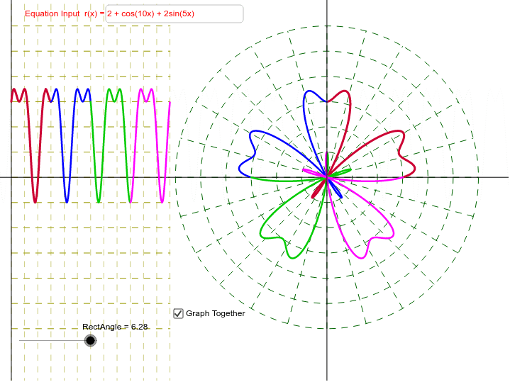
该范例展示了三角函数在直角坐标系和极坐标系中的图形。通过拖动直角坐标曲线,可以观察到其在两种坐标系下的变化。涉及的核心数学概念包括三角函数、直角坐标系和极坐标系。使用了CurveCartesian、Sequence、If等GeoGebra命令。适合高中数学教学和学习。
GeoGebra 命令及参数
Textfield(r) → inputBox1Line((0, 0), (1, 0)) → HorizAxisLine((0, 0), (0, 1)) → VertAxisSequence(Line[(a, 0), (a, 1)], a, 0, 6.28319, 0.5235987755982988) → VerticalLinesSequence(Circle[(12.5, 0), k], k, 1, 6) → polarCirclesSequence(Segment[(((-6) * cos(a)) + 12.5, ((-6) * sin(a))), ((6 * cos(a)) + 12.5, (6 * sin(a)))], a, 0, 2.87979, 0.2618) → radialLinesSequence(Segment[(0, a), (6.3, a)], a, -6, 6) → HorizontalLinesLine((12.5, 0), (12.5, 1)) → v_2If(a_2, RectAngle, PolarAngle) → PAMIf(a_2, PAM = RectAngle, PAM = PolarAngle) → bCurveCartesian((r(t) * cos(t)) + 12.5, (r(t) * sin(t)), t, 0, 6.283185307179586) → aCurveCartesian((r(t) * cos(t)) + 12.5, (r(t) * sin(t)), t, 0, Min[1.5707963267948966, PAM]) → a1CurveCartesian((r(t) * cos(t)) + 12.5, (r(t) * sin(t)), t, 1.5707963267948966, Min[3.141592653589793, PAM]) → a2CurveCartesian((r(t) * cos(t)) + 12.5, (r(t) * sin(t)), t, 3.141592653589793, Min[4.71238898038469, PAM]) → a3CurveCartesian((r(t) * cos(t)) + 12.5, (r(t) * sin(t)), t, 4.71238898038469, Min[6.283185307179586, PAM]) → a4