
球体扫描 by Juan Carlos Ponce Campuzano
几何画板及绘图内容加载中,请稍等……
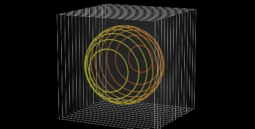
①本范例演示了球体与平面、多边形等几何元素的交互扫描过程,生成独特的数学艺术图形;②涉及的核心数学概念包括立体几何、导数、线性回归、参数方程、变换等;③作图要点提炼自构造摘要,使用了Polygon(多边形)、Translate(平移)、Sphere(球体)、Plane(平面)、IntersectPath(路径相交)等GeoGebra命令与对象;④适合高中及以上学生及数学爱好者学习空间几何、参数方程及数学艺术创作。
GeoGebra 命令及参数
Polygon(A, B, D, C) → p0, f, g, h, iTranslate(p0, Vector[(0, -1, 0), (0, (2 / n * (1 - 1)) - 1, 0)]) → P1Translate(p0, Vector[(0, -1, 0), (0, (2 / n * (2 - 1)) - 1, 0)]) → P2Translate(p0, Vector[(0, -1, 0), (0, (2 / n * (3 - 1)) - 1, 0)]) → P3Translate(p0, Vector[(0, -1, 0), (0, (2 / n * (4 - 1)) - 1, 0)]) → P4Translate(p0, Vector[(0, -1, 0), (0, (2 / n * (5 - 1)) - 1, 0)]) → P5Translate(p0, Vector[(0, -1, 0), (0, (2 / n * (6 - 1)) - 1, 0)]) → P6Translate(p0, Vector[(0, -1, 0), (0, (2 / n * (7 - 1)) - 1, 0)]) → P7Translate(p0, Vector[(0, -1, 0), (0, (2 / n * (8 - 1)) - 1, 0)]) → P8Translate(p0, Vector[(0, -1, 0), (0, (2 / n * (9 - 1)) - 1, 0)]) → P9Translate(p0, Vector[(0, -1, 0), (0, (2 / n * (10 - 1)) - 1, 0)]) → P10Translate(p0, Vector[(0, -1, 0), (0, (2 / n * (11 - 1)) - 1, 0)]) → P11Translate(p0, Vector[(0, -1, 0), (0, (2 / n * (12 - 1)) - 1, 0)]) → P12Translate(p0, Vector[(0, -1, 0), (0, (2 / n * (13 - 1)) - 1, 0)]) → P13Translate(p0, Vector[(0, -1, 0), (0, (2 / n * (14 - 1)) - 1, 0)]) → P14Translate(p0, Vector[(0, -1, 0), (0, (2 / n * (15 - 1)) - 1, 0)]) → P15Sphere((0, t, 0), 0.75) → sPlane(P1) → PO1Plane(P2) → PO2Plane(P3) → PO3Plane(P4) → PO4Plane(P5) → PO5Plane(P6) → PO6Plane(P7) → PO7Plane(P8) → PO8Plane(P9) → PO9Plane(P10) → PO10Plane(P11) → PO11Plane(P12) → PO12Plane(P13) → PO13Plane(P14) → PO14Plane(P15) → PO15IntersectPath(PO1, s) → S1IntersectPath(PO2, s) → S2IntersectPath(PO3, s) → S3IntersectPath(PO4, s) → S4IntersectPath(PO5, s) → S5IntersectPath(PO6, s) → S6IntersectPath(PO7, s) → S7IntersectPath(PO8, s) → S8IntersectPath(PO9, s) → S9IntersectPath(PO10, s) → S10IntersectPath(PO11, s) → S11IntersectPath(PO12, s) → S12IntersectPath(PO13, s) → S13IntersectPath(PO14, s) → S14IntersectPath(PO15, s) → S15