
线性相关系数比较演示
几何画板及绘图内容加载中,请稍等……
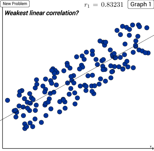
① 本范例演示两组随机散点图的线性相关系数对比,直观展示相关强弱差异。② 核心数学概念包括线性相关、皮尔逊相关系数、线性回归拟合、散点分布特征。③ 作图要点:使用 Sequence 生成随机点序列,If 判断条件,PMCC 计算相关系数,FitLineY 拟合回归线,LaTeX 显示公式,AxisStepX 设置坐标轴刻度;对象涉及 l_0、type_1、xrnd_1、elem_1、l_n、l_p、corner1、corner3、strength_1、L_1、pts_1、r_1 等。④ 适合高中统计与概率课程、大学入门统计教学及数据分析入门演示。
GeoGebra 命令及参数
Sequence((2 * random()) - 1 + i, i, 1.5, 15.9, 0.1) → xrnd_1If(type_1 ≟ 0, Element[l_0, elem_1], If[type_1 < 0, Element[l_n, elem_1], Element[l_p, elem_1]]) → L_1Sequence((Element[xrnd_1, j], ((((elem_1 + 2) * 2) * random()) - (elem_1 + 2)) / strength_1 + L_1(Element[xrnd_1, j])), j, 1, Length[xrnd_1]) → pts_1PMCC(pts_1) → r_1FitLineY(pts_1) → reg_1Sequence((2 * random()) - 1 + i, i, 1.5, 15.9, 0.1) → xrnd_2If(type_2 ≟ 0, Element[l_0, elem_2], If[type_2 < 0, Element[l_n, elem_2], Element[l_p, elem_2]]) → L_2Sequence((Element[xrnd_2, j], ((((elem_2 + 2) * 2) * random()) - (elem_2 + 2)) / strength_2 + L_2(Element[xrnd_2, j])), j, 1, Length[xrnd_2]) → pts_2FitLineY(pts_2) → reg_2PMCC(pts_2) → r_2LaTeX(r_1, true, true) → txtr1LaTeX(r_2, true, true) → txtr2AxisStepX() → xx
AI 绘图提示语参考
绘制一个统计图表,用于并排比较两个随机散点图的线性相关系数,以可视化相关强度的差异。图表包含两个散点图,每个由一组随机生成的点构成,并配有拟合的回归线。每个散点图旁用公式形式显示其Pearson相关系数,图表设置轴步长以确保清晰。构造顺序为先生成随机点集,再计算相关系数与回归线,最后渲染公式。
以上提示语为根据原始绘图命令整理而来,仅供参考。