
解线性方程组的几何方法
几何画板及绘图内容加载中,请稍等……
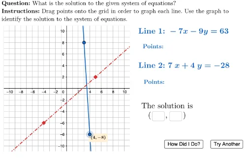
本范例演示如何通过几何方法解线性方程组。核心数学概念包括线性方程组的图形表示和交点。使用GeoGebra命令包括Point, Element, Polygon, Line, Intersect等。适合初中及以上学生学习线性代数和解析几何。
GeoGebra 命令及参数
Point({userPOIx, userPOIy}) → userPOIElement(questionList, questionListIndex) → questionNumElement(C2:C5, questionNum) → poiPolygon({(-11, -11), (-11, 11), (11, 11), (11, -11)}) → viewBoxLaTeX((((("\text{" * QUESTION) * "\\") * INSTRUCTIONS) * "}")) → TEXTDynamicCoordinates(free1A, If[IsInRegion[free1A, viewBox], x(free1A), 18.5], If[IsInRegion[free1A, viewBox], y(free1A), 7.25]) → line1ADynamicCoordinates(free2A, If[IsInRegion[free2A, viewBox], x(free2A), 18.5], If[IsInRegion[free2A, viewBox], y(free2A), 1.25]) → line2ADynamicCoordinates(free2B, If[IsInRegion[free2B, viewBox], x(free2B), 20.5], If[IsInRegion[free2B, viewBox], y(free2B), 1.25]) → line2BDynamicCoordinates(free1B, If[IsInRegion[free1B, viewBox], x(free1B), 20.5], If[IsInRegion[free1B, viewBox], y(free1B), 7.25]) → line1BLine(line1A, line1B) → userLine1Line(line2A, line2B) → userLine2Intersect(A2, B2) → C2Intersect(A3, B3) → C3Intersect(A4, B4) → C4Intersect(A5, B5) → C5Element(A2:A5, questionNum) → line1Element(B2:B5, questionNum) → line2LaTeX(("\text{Line 1: }" * line1)) → labelLine1LaTeX(("\text{Line 2: }" * line2)) → labelLine2LaTeX("\text{Points: }") → pointsLine1LaTeX("\text{Points: }") → pointsLine2Textfield(textPOIx) → ansBoxXTextfield(textPOIy) → ansBoxYLaTeX("\begin{tabular}{c}\text{The solution is}\\(\hspace{45},\hspace{45})\end{tabular}") → solutionLaTeX(activePoint) → activePointLabelLaTeX(poi) → poiLabelLaTeX("\text{Line 1}") → line1LabelOnGridLaTeX("\text{Line 2}") → line2LabelOnGrid
AI 绘图提示语参考
在一个坐标系的网格中绘制两条直线,并标示它们的交点。首先,在坐标系内绘制一个边框,然后画出两条直线,并动态调整它们的位置,确保它们在边框内显示。接着,找到两条直线的交点,并用不同的颜色或标记标示出来。最后,在图中添加文字说明,标明两条直线的方程和交点的坐标。
以上提示语为根据原始绘图命令整理而来,仅供参考。