
分布载荷的力学分析
几何画板及绘图内容加载中,请稍等……
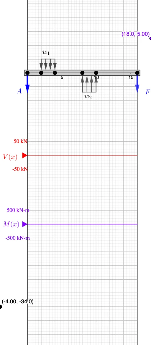
①本范例演示了分布载荷在梁上的力学效应与弯矩分布;②涉及的核心数学概念包括积分、导数、向量运算和几何作图;③作图要点:使用Point, Vector, If, Sort, Max, Min, member, Segment, Textfield, Polygon, Sequence等GeoGebra命令和对象构建载荷分布、梁体及力学分析图形;④适合高中及以上学生及工程技术人员学习结构力学与微积分应用。
GeoGebra 命令及参数
Point(xAxis) → CPoint(xAxis) → BPoint(xAxis) → AVector(A, Midpoint[B, C]) → r_{w_1}Point(xAxis) → EPoint(xAxis) → FVector(A, F) → r_FPoint(xAxis) → DVector(A, Midpoint[E, D]) → r_{w2}If(abs(w_1) > abs(w_2), {1.4, 1}, If[abs(w_1) < abs(w_2), {1, 1.4}, {1, 1}]) → heightIf(x(D) < x(E), D, E) → startIf(start ≟ D, E, D) → endVector(A, C) → r_{P_1}Sort(Unique[x({A, B, C, D, E, F})]) → pointsVector(A, B) → r_BMax(x({A, C, B, D, E, F})) → rightPoint(x = ((-AxisStepX[])) / 4) → VMin(x({A, C, B, D, E})) → leftIf(w_2 < 0, Polygon[E + (0.2 * j), E + (height(2) * j), D + (height(2) * j), D + (0.2 * j)], Mirror[Polygon[E + (0.2 * j), E + (height(2) * j), D + (height(2) * j), D + (0.2 * j)], xAxis]) → load_2member(A, (right, 0), (0.2 * AxisStepY[])) → beam, beam_t, beam_b, beam_r, beam_LSegment((x(A), v'(x(A))), (x(A), v'(x(A) + 0.001))) → v_ASegment((x(B), v'(x(B))), (x(B), v'(x(B) + 0.001))) → v_BPoint(x = ((-AxisStepX[])) / 4) → MSegment((x(C), v'(x(C))), (x(C), v'(x(C) + 0.001))) → v_CSegment(V', (x(V'), v'(right))) → v_rMax(Join[{{0}, y(Sequence[Max[m, points(k), points(k + 1)], k, 1, Length[points] - 1])}]) → M_{max}Min(Join[{{0}, y(Sequence[Min[v, points(k), points(k + 1)], k, 1, Length[points] - 1])}]) → V_{min}Textfield(Scale_V) → InputBox1Textfield(Scale_M) → InputBox2Polygon((right, y(Corner[2])), (right, y(Corner[3])), Corner[3], Corner[2]) → mask, mask_l, mask_t, mask_r, mask_bSegment((0, y(V)), (right, y(V))) → VaxisSegment((0, y(M)), (right, y(M))) → MaxisMax(Join[{{0}, y(Sequence[Max[v, points(k), points(k + 1)], k, 1, Length[points] - 1])}]) → V_{max}Min(Join[{{0}, y(Sequence[Min[m, points(k), points(k + 1)], k, 1, Length[points] - 1])}]) → M_{min}If(w_1 < 0, Polygon[B + (0.2 * j), B + (height(1) * j), C + (height(1) * j), C + (0.2 * j)], Mirror[Polygon[B + (0.2 * j), B + (height(1) * j), C + (height(1) * j), C + (0.2 * j)], xAxis]) → load_1If(F_A ≥ 0, Vector[A - (1.5 * j), A], Vector[A, A - (1.5 * j)]) → aIf(F_F ≥ 0, Vector[F - (1.5 * j), F], Vector[F, F - (1.5 * j)]) → fSequence(Vector[If[w_1 < 0, Vector[B + (height(1) * j) + (n * delta), B + (0.2 * j) + (n * delta)], Vector[B - (height(1) * j) + (n * delta), B - (0.2 * j) + (n * delta)]]], n, 0, Length[Segment[B, C]] / abs(delta)) → distLoad_1Sequence(Vector[If[w_2 < 0, Vector[D + (height(2) * j) + (n * delta), D + (0.2 * j) + (n * delta)], Vector[D - (height(2) * j) + (n * delta), D - (0.2 * j) + (n * delta)]]], n, 0, Length[Segment[D, E]] / abs(delta)) → distLoad_2Segment((x(F), v'(x(F))), (x(F), v'(x(F) + 0.001))) → v_F
AI 绘图提示语参考
绘制一个悬臂梁,在梁上施加两个分布载荷,分别位于梁的两端。使用向量表示载荷的方向和大小,通过点和向量构造梁的几何形状。计算并显示梁上最大和最小弯矩及剪力值,以及梁的边界条件。绘制梁的受力图,包括剪力图和弯矩图。
以上提示语为根据原始绘图命令整理而来,仅供参考。