
Volume Under a Surface Rectangular Solid Approximation
Loading the math board and drawing, please wait…
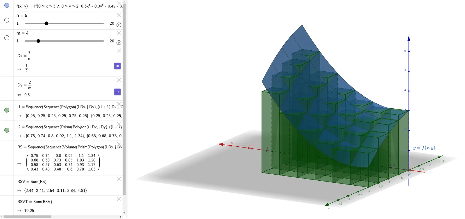
This example demonstrates the geometric concept of approximating the volume under a surface using rectangular solids. It involves core mathematical concepts like surface, volume, variance, limits, means, addition, and differential calculus. The construction utilizes GeoGebra commands such as Sequence and Sum, along with objects like function f, parameters n and m, increments Dx and Dy, lengths l1 and l2, and components like RS (rectangular solid volume), RSV (sum of volumes), and RSVT (actual volume). It is suitable for high school and above, particularly for visualizing the process of volume calculation in multivariable calculus and integral theory.
GeoGebra Commands & Parameters
Sequence(Sequence[Polygon[((i * Dx), (j * Dy)), (((i + 1) * Dx), (j * Dy)), (((i + 1) * Dx), ((j + 1) * Dy)), ((i * Dx), ((j + 1) * Dy))], i, 0, n - 1], j, 0, m - 1) → l1Sequence(Sequence[Prism[Polygon[((i * Dx), (j * Dy)), (((i + 1) * Dx), (j * Dy)), (((i + 1) * Dx), ((j + 1) * Dy)), ((i * Dx), ((j + 1) * Dy))], f((i * Dx), (j * Dy))], i, 0, n - 1], j, 0, m - 1) → l2Sequence(Sequence[Volume[Prism[Polygon[((i * Dx), (j * Dy)), (((i + 1) * Dx), (j * Dy)), (((i + 1) * Dx), ((j + 1) * Dy)), ((i * Dx), ((j + 1) * Dy))], f((i * Dx), (j * Dy))]], i, 0, n - 1], j, 0, m - 1) → RSSum(RS) → RSVSum(RSV) → RSVT
AI Drawing Prompt Reference
Draw the approximation of the volume under a surface using rectangular solids. First, create a grid of rectangles with vertices determined by parameters Dx and Dy. Then, build rectangular prisms with each rectangle as the base and the height determined by the function f. Next, calculate the volume of each prism, and finally sum up all the volumes to get the approximate volume.
The prompt above was compiled from the original drawing commands and is for reference only.