
Volume by Cylindrical Shells - Example sin(x^2)
Loading the math board and drawing, please wait…
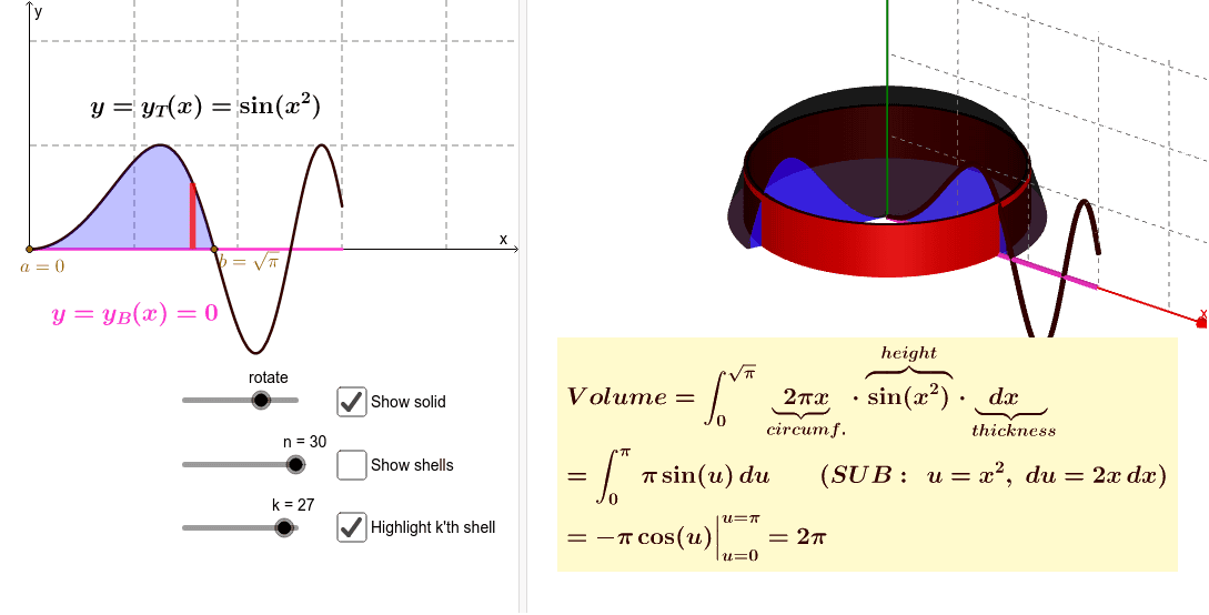
This example demonstrates the volume of a solid of revolution using the method of cylindrical shells for the function sin(x^2). It covers the application of integration in geometry, including the cylindrical shell method and volume calculation. It uses commands like Sequence, Surface, Polygon, Segment in GeoGebra, suitable for high school mathematics education.
GeoGebra Commands & Parameters
Sequence(a + ((k - 0.5) * dx), k, 1, n) → midptsSequence(a + (k * dx), k, 0, n - 1) → leftptsSequence(a + (k * dx), k, 1, n) → rightptsSequence(Polygon[(xk(k - 1), y_B(Element[evalpts, k])), (xk(k - 1), y_T(Element[evalpts, k])), (xk(k), y_T(Element[evalpts, k])), (xk(k), y_B(Element[evalpts, k]))], k, 1, n) → RectanglesSequence((Element[evalpts, k], 0), k, 1, n) → evalptsplotSurface(xrot + ((xk(k - 1) - xrot) * cos(t)), h, ((xk(k - 1) - xrot) * sin(t)), t, 0, (2 * π), h, y_B(Element[evalpts, k]), y_T(Element[evalpts, k])) → ShellIn_kSurface(xrot + (r * cos(t)), y_T(Element[evalpts, k]), (r * sin(t)), t, 0, (2 * π), r, xk(k - 1) - xrot, xk(k) - xrot) → UpShell_kSurface(xrot + ((xk(k) - xrot) * cos(t)), h, ((xk(k) - xrot) * sin(t)), t, 0, (2 * π), h, y_B(Element[evalpts, k]), y_T(Element[evalpts, k])) → ShellOut_kSurface(xrot + (r * cos(t)), y_B(Element[evalpts, k]), (r * sin(t)), t, 0, (2 * π), r, xk(k - 1) - xrot, xk(k) - xrot) → ShellDown_kSequence(Surface[xrot + ((xk(k - 1) - xrot) * cos(t)), h, ((xk(k - 1) - xrot) * sin(t)), t, 0, (2 * π), h, y_B(Element[evalpts, k]), y_T(Element[evalpts, k])], k, 1, n) → ShellsInSequence(Surface[xrot + (r * cos(t)), y_T(Element[evalpts, k]), (r * sin(t)), t, 0, (2 * π), r, xk(k - 1) - xrot, xk(k) - xrot], k, 1, n) → ShellsUpSequence(Surface[xrot + (r * cos(t)), y_B(Element[evalpts, k]), (r * sin(t)), t, 0, (2 * π), r, xk(k - 1) - xrot, xk(k) - xrot], k, 1, n) → ShellsDownSequence(Surface[xrot + ((xk(k) - xrot) * cos(t)), h, ((xk(k) - xrot) * sin(t)), t, 0, (2 * π), h, y_B(Element[evalpts, k]), y_T(Element[evalpts, k])], k, 1, n) → ShellsOutSurface(xrot + (cos((-t)) * (u - xrot)), y_B(u), (sin((-t)) * (u - xrot)), u, a, b, t, 0, RotationAngle) → Solid_BSurface(xrot + (cos((-t)) * (u - xrot)), y_T(u), (sin((-t)) * (u - xrot)), u, a, b, t, 0, RotationAngle) → Solid_TSurface(xrot + ((a - xrot) * cos((-t))), h, ((a - xrot) * sin((-t))), t, 0, RotationAngle, h, y_B(a), y_T(a)) → Solid_aSurface(xrot + ((b - xrot) * cos((-t))), h, ((b - xrot) * sin((-t))), t, 0, RotationAngle, h, y_B(b), y_T(b)) → Solid_bSurface(xrot + (cos((-RotationAngle)) * (u - xrot)), ((1 - w) * y_B(u)) + (w * y_T(u)), (sin((-RotationAngle)) * (u - xrot)), w, 0, 1, u, a, b) → Solid_eSurface(xrot + u - xrot, ((1 - w) * y_B(u)) + (w * y_T(u)), (0 * (u - xrot)), w, 0, 1, u, a, b) → region3dPolygon((xk(k - 1), y_B(Element[evalpts, k])), (xk(k - 1), y_T(Element[evalpts, k])), (xk(k), y_T(Element[evalpts, k])), (xk(k), y_B(Element[evalpts, k]))) → Rectangle_k, f, g, h, iSegment((0, 0), (xrot, 0)) → c