
Visualizing the Mean Value Theorem for Integral and its Proofs
Loading the math board and drawing, please wait…
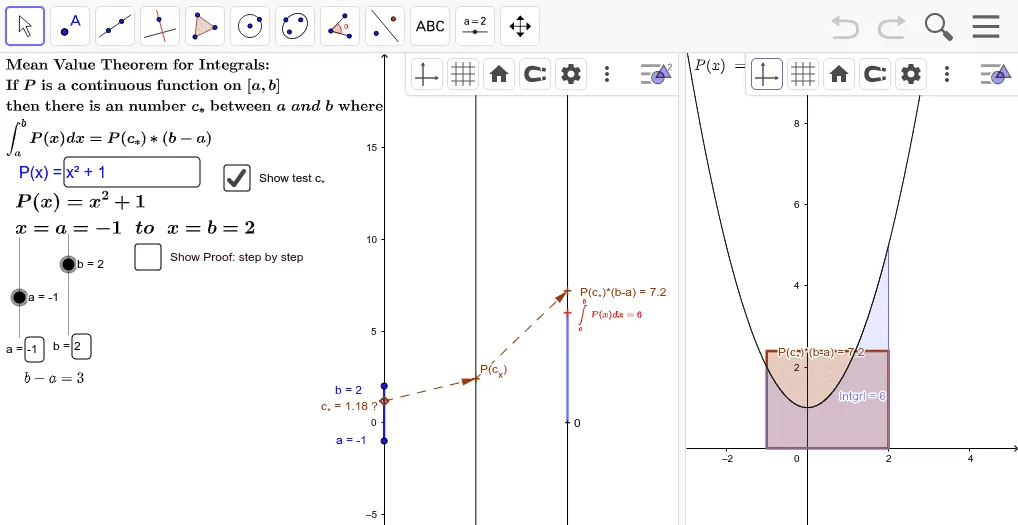
This example visualizes the Mean Value Theorem for Integrals using mapping diagrams and graphs, outlining the proof. Key math concepts include integrals, averages, and function graphs. GeoGebra commands like Integral, Intersect, Extremum, etc., are used in construction. Suitable for high school and above mathematics learners to understand the theorem and its applications.
GeoGebra Commands & Parameters
Integral(P, a, b) → IntgrlIntersect(P, e) → A, CExtremum(P, a, b) → M,Textfield(P) → inputBox1Textfield(a) → inputBox2Textfield(b) → inputBox3Max({y(M), P(a), P(b)}) → MAXMin({y(M), P(a), P(b)}) → MINVector(Max_{f}, S_2) → uVector(Min_{f}, T_1) → vVector(Z_*, U_2) → wLine(Max_{f}, S_2) → hLine(U_2, Z_*) → iLine(T_1, Min_{f}) → jVector(C_*, Z_*) → zSegment(x_a, x_b) → kPoint(yAxis) → XVector(X, P_X) → lIntegral(Intgrl / (b - a), a, b) → mvtIntegral(MAX, a, b) → MaxRecIntegral(MIN, a, b) → MinRecVector(P_X, CheckX) → rPolygon({(a, 0), a}) → poly1Polygon({(a, 0), (a, P(y(X))), (b, P(y(X))), (b, 0)}) → MVRecSegment(Max_{f}, Min_{f}) → sSegment(P0, U_2) → t