
Visualizing Statistical Power of Hypothesis Tests
Loading the math board and drawing, please wait…
In collections
AP Statistics
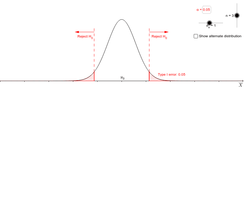
This example demonstrates the concept of statistical power visually, illustrating the relationship between power, sample size, and standard deviation in hypothesis testing. Key math concepts include hypothesis testing, statistical power, sample size, standard deviation, and normal distributions. It is constructed using GeoGebra commands like Point, InverseNormal, Normal, Segment, IntegralBetween, Textfield, and Vector, making it suitable for high school students and beginners in statistics learning hypothesis testing and power analysis.
GeoGebra Commands & Parameters
Point(baseline) → mu1PointInverseNormal(mu0, sigma0, 1 - alpha / 2) → nullRightThresholdInverseNormal(mu0, sigma0, alpha / 2) → nullLeftThresholdNormal(mu0, sigma0, x) → nullDistSegment((nullLeftThreshold, nullDist(nullLeftThreshold)), (nullLeftThreshold, 0)) → leftThresholdLineSegment((nullRightThreshold, nullDist(nullRightThreshold)), (nullRightThreshold, 0)) → rightThresholdLineIntegralBetween(f, baseline, nullLeftThreshold, nullRightThreshold) → T2RegionIntegralBetween(f, baseline, Min[leftBound, mu1 - (4 * sigma1)], nullLeftThreshold) → leftPowerRegionIntegralBetween(f, baseline, nullRightThreshold, Max[rightBound, mu1 + (4 * sigma1)]) → rightPowerRegionTextfield(alpha) → alphaInputBoxIntegralBetween(nullDist, 0, leftBound, nullLeftThreshold) → t1lefttailIntegralBetween(nullDist, 0, nullRightThreshold, rightBound) → t1righttailSegment((nullLeftThreshold, nullDist(nullLeftThreshold)), (nullLeftThreshold, 0.6)) → leftRejectLineSegment((nullRightThreshold, nullDist(nullRightThreshold)), (nullRightThreshold, 0.6)) → rightRejectLineVector((nullLeftThreshold, 0.55), (nullLeftThreshold - 0.8, 0.55)) → leftRejectArrowVector((nullRightThreshold, 0.55), (nullRightThreshold + 0.8, 0.55)) → rightRejectArrowTextfield(difference) → differenceInputBoxSegment((nullLeftThreshold, 0), (nullLeftThreshold, offset)) → leftThresholdLine2Segment((nullRightThreshold, 0), (nullRightThreshold, offset)) → rightThresholdLine2Segment(Point[{mu0, offset - 0.09}], Point[{mu0, offset - 0.11}]) → differenceLineLeftEndSegment(Point[{mu1, offset - 0.09}], Point[{mu1, offset - 0.11}]) → differenceLineRightEndSegment(Point[{mu0, offset}], Point[{mu0, offset - 0.017}]) → altOriginMarkSegment((mu0, 0), (mu0, offset)) → mu0GuidelineVector((mu0, offset - 0.1), (mu1, offset - 0.1)) → differenceLine
AI Drawing Prompt Reference
Create a visualization of statistical power in hypothesis tests, featuring horizontal lines for critical values, a normal distribution curve, and integral regions for type I and type II errors. Use sliders to adjust standard deviation and sample size, showing how power changes with different parameters. Include arrows and text annotations to label key areas and parameters.
The prompt above was compiled from the original drawing commands and is for reference only.