
Visualizing Pythagoras Theorem
Loading the math board and drawing, please wait…
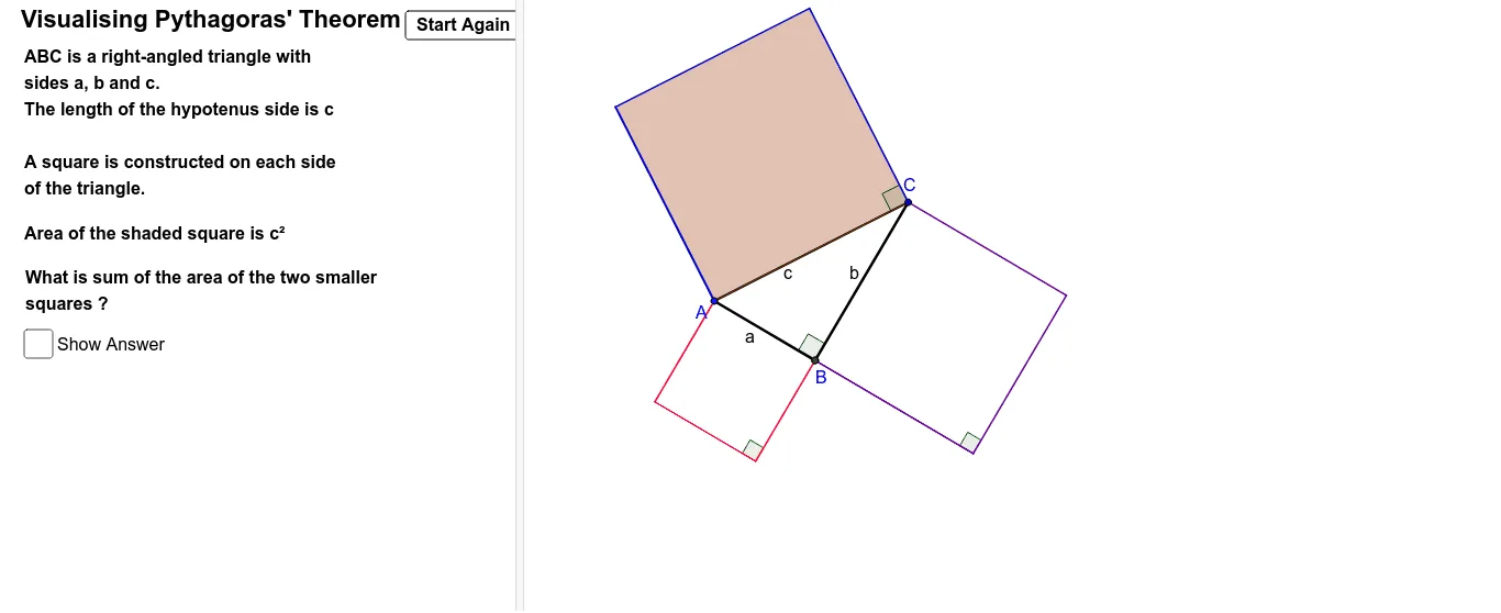
This example dynamically demonstrates the relationship between the sides of a right triangle, visually showcasing the geometric meaning of Pythagoras' Theorem. Core math concepts include Pythagorean Theorem, right triangles, and side length calculations. Construction highlights involve commands like Segment, OrthogonalLine, Point, Polygon, Line, Intersect, Angle, Random, and objects such as M, ycorN, xcorN, A, B, a, b_3, C, c, b, etc. Ideal for middle school and above learners to grasp the theorem and its applications.
GeoGebra Commands & Parameters
Segment(A, B) → aOrthogonalLine(B, a) → b_3Point(b_3) → CSegment(A, C) → cSegment(C, B) → bPolygon(B, A, 4) → poly1, e, f, g, h, D, EPolygon(A, C, 4) → poly2, i, j, k, l, F, GPolygon(C, B, 4) → poly3, m, n, p, q, H, ILine(P, c) → rIntersect(r, j) → JSegment(A, G) → s_1Segment(G, F) → a_1Segment(F, C) → b_1Polygon(A, C, J, P) → poly4, a_2, c_1, j_1, p_1Segment(A, D) → d_1Segment(D, E) → e_1Segment(E, B) → f_1Segment(B, H) → g_1Segment(H, I) → h_1Segment(I, C) → i_1Line(Q, e_1) → k_1Intersect(k_1, f_1) → KPolygon(D, E, K, Q) → poly5, d_2, e_2, k_2, q_1Line(R, g_1) → l_1Intersect(l_1, h_1) → LPolygon(B, H, L, R) → poly6, b_2, h_2, l_2, r_1Angle(C, B, A) → αAngle(F, C, A) → βAngle(B, E, D) → γAngle(I, H, B) → δSegment(M, N) → m_1OrthogonalLine(N, m_1) → n_1Point(n_1) → OSegment(M, O) → t_1Segment(O, N) → c_2Random(1, 3) → sideAngle(O, N, M) → ε
AI Drawing Prompt Reference
Visualize the Pythagorean theorem by drawing a right triangle with its three sides dynamically linked, fill the areas of the two smaller squares on the legs and the larger square on the hypotenuse, measure angles and use random side lengths, and construct additional geometric figures to demonstrate the theorem's proof.
The prompt above was compiled from the original drawing commands and is for reference only.