Visualizing Polynomial Roots with Extrema and Turning Points

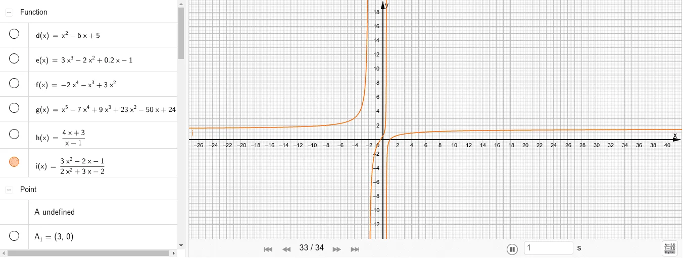
This example demonstrates how to link a polynomial assignment with its computed roots and key shape-defining points (extrema and turning points) in one interactive graphing environment. It focuses on the geometric meaning of polynomial zeros and how they relate to the curve’s behavior. The core concepts are: polynomial roots (solutions where the function equals zero), extrema (local maxima/minima), and turning points (points where the curve changes its monotonicity/curvature trend). Construction-wise, it uses GeoGebra commands Root to compute and display the roots of the relevant functions, Extremum to locate and mark extrema, and TurningPoint to identify turning points on the polynomial curves. Multiple function objects (e.g., f, g, h) and many derived point/curve objects (e.g., A, B, C, …, plus indexed variants like A_1, B_1, …) are used to build and relate the curves and their critical points, producing a clear visualization of how algebraic solutions correspond to visible features of the graphs. Suitable for high school to early undergraduate teaching, especially for function graph analysis and intuitive groundwork before formal calculus topics.