Visualizing Limits for Complex Functions

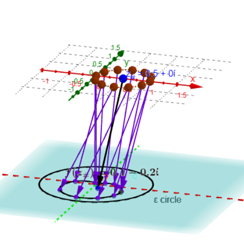
This GeoGebra example dynamically illustrates the limit of a complex function in the complex plane, showing how f(z) approaches a limit L as z tends to a point. It emphasizes the ε-δ definition of complex limits, path independence, and the behavior of function values near the limit point. The construction uses commands such as Sequence, Zip, If, Circle, Line, Vector, Point, Locus, and Textfield to create interactive ε-circles, δ-neighborhoods, and traced function-value paths. Objects include dynamic sliders for ε and δ, input boxes for parameters, and loci of f(z) along various approach paths. This is ideal for university-level complex analysis courses, helping students grasp the geometric meaning of limits in the complex domain and compare with real-variable limits. It also serves as a powerful visual aid for instructors and self-learners in advanced calculus or mathematical visualization.