
Visualizing Complex Roots of Polynomials by Mark Dabbs
Loading the math board and drawing, please wait…
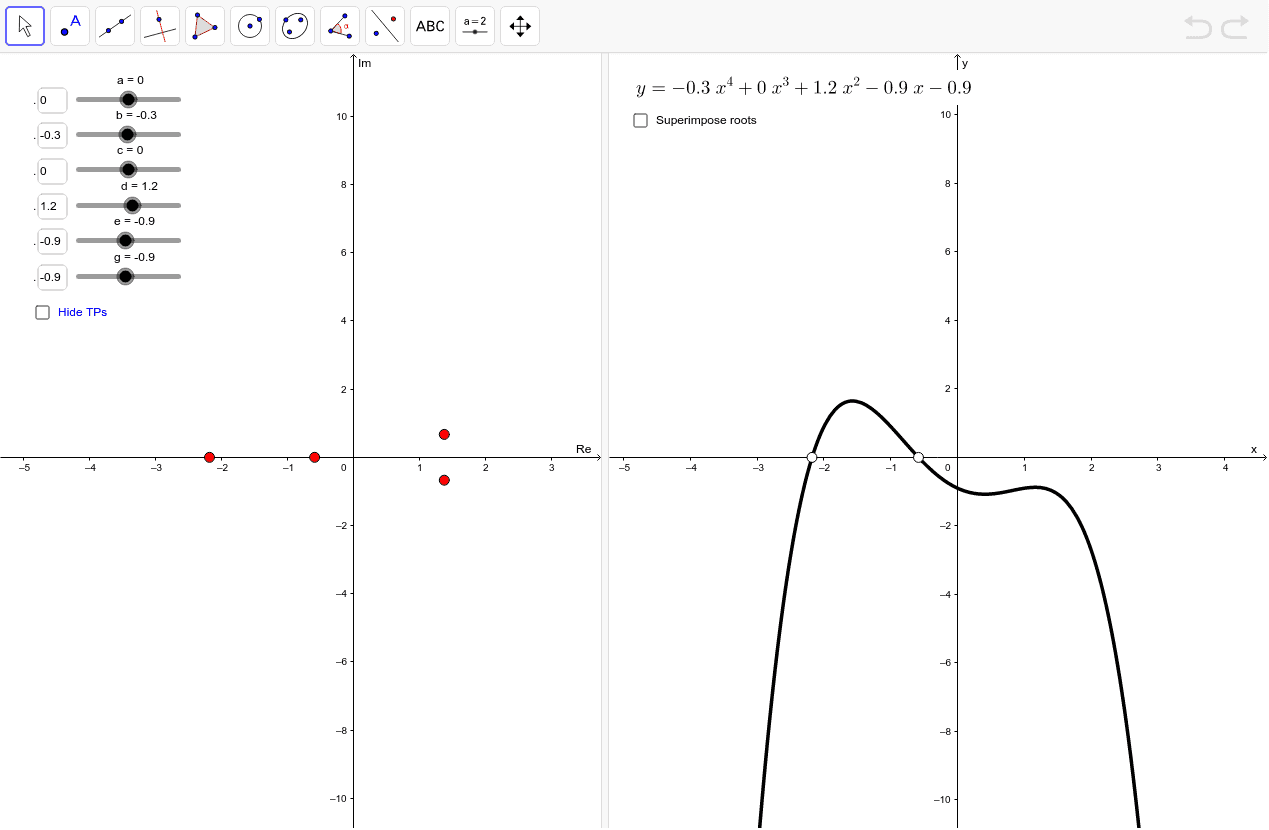
This example dynamically visualizes the complex roots of polynomials. It involves key mathematical concepts such as polynomial functions, complex numbers, and trigonometric functions. Using GeoGebra commands like If, Sequence, and Textfield, users can observe how the roots of a polynomial change with parameter variations. Suitable for high school mathematics education and learning.
GeoGebra Commands & Parameters
If(a ≠ 0, myFA, If[b ≠ 0, myFB, If[c ≠ 0, myFC, If[d ≠ 0, myFD, If[e ≠ 0, myFE, If[e ≠ 0, myFE, myFG]]]]]) → fxSequence(x = x(Element[myTPsA, k]), k, 1, Length[myTPsA]) → vTPLinesASequence(x = x(Element[myTPsA, k]), k, 1, Length[myTPsA]) → Lines2Textfield(a) → inputBox1Textfield(b) → inputBox2Textfield(c) → inputBox3Textfield(d) → inputBox4Textfield(e) → inputBox5Textfield(g) → inputBox6
AI Drawing Prompt Reference
Create a dynamic visualization of the complex roots of a polynomial. Input the coefficients a, b, c, d, and e, then display the polynomial graph and its complex roots dynamically. Adjust the coefficients using sliders to observe the changes in the roots.
The prompt above was compiled from the original drawing commands and is for reference only.