Visualizing a System of Linear Equations: Intersection of Two Lines by Alan Chan

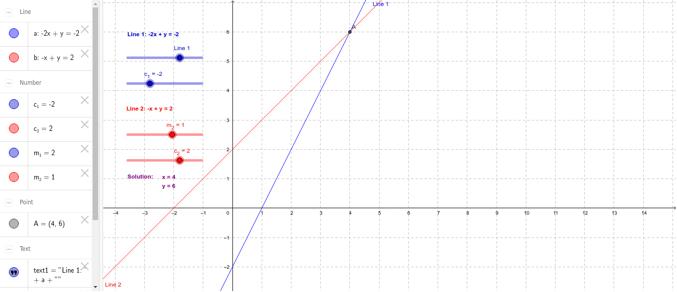
① This example dynamically demonstrates how the solution of a system of two linear equations (the intersection point of two lines) changes as the slopes and intercepts are adjusted. ② Core mathematical concepts include linear equations, slope-intercept form (y = mx + c), systems of equations, intersection points, and parametric effects on solutions. ③ Construction: Using GeoGebra commands Line and Intersect, two lines are created with parameters m_1, c_1, m_2, c_2; the intersection point A is computed, and text objects (text1–text4) display the equations and solution. Sliders (a, b) likely control parameter values. ④ Suitable for middle and high school students learning algebra and coordinate geometry, as well as teachers for classroom demonstrations, helping visualize unique, no, or infinite solutions from a geometric perspective.