Graphical Method for Solving Polynomial Inequalities

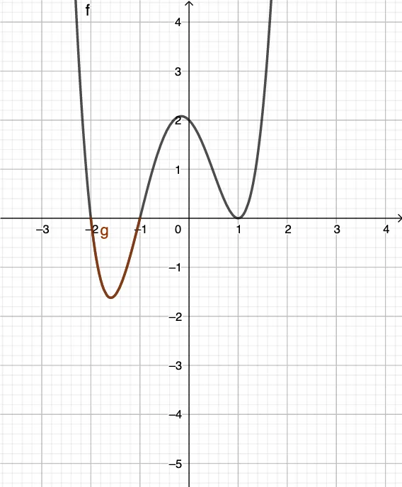
This example demonstrates how to solve one-variable polynomial inequalities by graphing. By plotting a polynomial function and visually comparing it to the x-axis, learners can determine where the inequality holds (e.g., f(x) > 0 or f(x) ≤ 0) and read the solution intervals directly from the graph. The key mathematical ideas include polynomial functions, roots/zeros, sign analysis, and interpreting inequalities using graph positions relative to the x-axis. Construction-wise, the GeoGebra setup uses function-related objects such as f and g: f represents the polynomial, while g is used to display the corresponding graph and support the reading of critical points. The solution is obtained by locating x-intercepts (where f crosses or touches the x-axis) and then determining the sign of the function on each interval separated by these roots. Suitable for high-school to pre-college students, it supports classroom visualization and self-study of inequality-solving techniques via graphing.