
Visualization of Riemann Sum in 3D Space
Loading the math board and drawing, please wait…
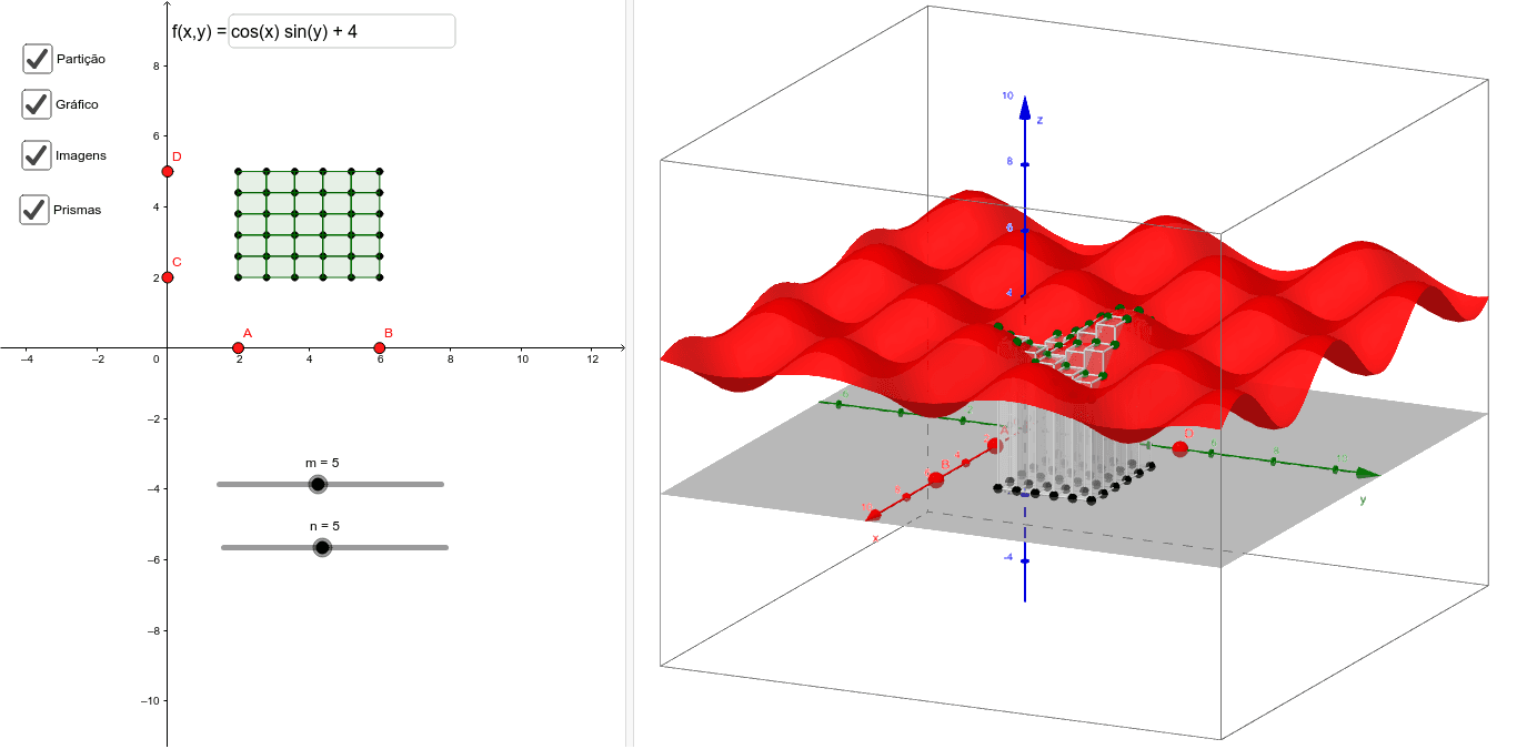
This example visualizes the Riemann sum approximation for volume under a surface in 3D space. Core concepts include multiple integrals, Riemann sums, and solid geometry volume estimation. Construction utilizes GeoGebra commands like Sequence for grid generation, Polygon for prism building, and Point/Min/Max for boundary definition. Suitable for high school math extension or university calculus courses to intuitively understand the geometric meaning of double integrals.
GeoGebra Commands & Parameters
Point(xAxis) → APoint(xAxis) → BMin(x(B), x(A)) → xminMax(x(B), x(A)) → xmaxPoint(yAxis) → CPoint(yAxis) → DMax(y(C), y(D)) → ymaxMin(y(C), y(D)) → yminSequence(Sequence[(xmin + (dx * i), ymin + (dy * j)), i, 0, m], j, 0, n) → lista3Polygon((xmin, ymin), (xmax, ymin), (xmax, ymax), (xmin, ymax)) → R, a, b, c, dSequence(Sequence[(xmin + (dx * i), ymin + (dy * j), f(xmin + (dx * i), ymin + (dy * j))), i, 0, m], j, 0, n) → ImagensSequence(Sequence[Polygon[Element[Element[lista3, j], i], Element[Element[lista3, j], i + 1], Element[Element[lista3, j + 1], i + 1], Element[Element[lista3, j + 1], i]], i, 1, m], j, 1, n) → PartSequence(Sequence[Prism[Element[Element[Part, i], j], Element[Element[Imagens, i], j]], j, 1, m], i, 1, n) → PrismasSequence((xmin + (dx * i), 0), i, 0, m) → lista1Sequence((0, ymin + (dy * i)), i, 0, n) → lista2Textfield(f) → ct1
AI Drawing Prompt Reference
Visualize the Riemann sum approximation for the volume under a surface in 3D space. Start by defining two points on the x-axis and y-axis, and determine their minimum and maximum values to create a rectangular grid. Then, generate multiple quadrilaterals based on the function's values at grid points, each representing a small volume element. Stack prisms for each quadrilateral along its base to approximate the volume under the surface. Finally, label the function expression to illustrate its relationship with the geometric shape.
The prompt above was compiled from the original drawing commands and is for reference only.