
Volumes - Discs (Perpendicular to the x-axis)
Loading the math board and drawing, please wait…
In collections
Calculus - Applications of Integrals - Areas and Volumes
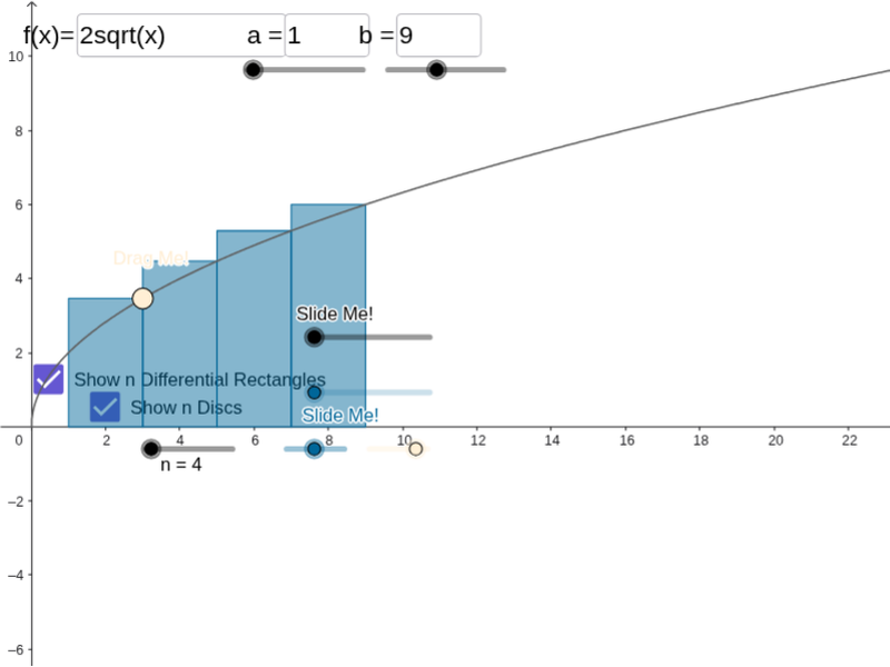
This example demonstrates the calculation of volumes of solids of revolution using the disc method. Core mathematical concepts include integral calculus, volume formulas for rotated bodies, and geometric transformations of function graphs. The construction utilizes GeoGebra commands and objects such as Sequence, Rotate, Intersect, Polygon, Circle, Surface, Cylinder, Dilate, Segment, Textfield, and Integral. It is suitable for high school and above students to understand the method of calculating volumes of solids of revolution and to visualize dynamic effects.
GeoGebra Commands & Parameters
Sequence(Polygon[(a + (i * deltax), 0), (a + ((i + 1) * deltax), 0), (a + ((i + 1) * deltax), f(a + ((i + 1) * deltax))), (a + (i * deltax), f(a + ((i + 1) * deltax)))], i, 0, n - 1, 1) → list1Rotate(list1, α, y = 0) → list1'Intersect(i, l) → BIntersect(k, l) → CIntersect(j, k) → DPolygon(C, B, A, D) → poly1, c_2, b_1, a_1, dRotate(C, α, y = 0) → C'Rotate(B, α, y = 0) → B'Rotate(A, α, y = 0) → A'Rotate(D, α, y = 0) → D'Polygon(C', B', A', D') → poly1', c', b', a', d'Sequence((a + (i * deltax), 0), i, 0, n, 1) → list2Sequence((a + (i * deltax), f(a + (i * deltax))), i, 1, n, 1) → list3Rotate(list3, α, y = 0) → list3'Sequence((a + (i * deltax), f(a + ((i + 1) * deltax))), i, 0, n - 1, 1) → list4Sequence(x = a + (i * deltax), i, 1, n, 1) → list6Sequence(Segment[Element[list3, i], Element[list4, i]], i, 0, n, 1) → list5Sequence(CircleSector[Element[list2, i + 1], Element[list3', i], Element[list3, i], xOyPlane], i, 1, n, 1) → list7Sequence(Cylinder[Element[list2, i], Element[list2, i + 1], f(Element[list2, i + 1])], i, 1, n, 1) → list8Sequence(Circle[Element[list2, i], f(Element[list2, i]), x = 0], i, 2, n + 1, 1) → list10Circle((a, 0), f(a + deltax), x = 0) → pSurface(q, α, xAxis) → eCylinder((x(A), 0), (x(A) - deltax, 0), y(A)) → o, r, s, tDilate(E, If[0 < u ≤ 1, 1 - u, 0], D) → E'Dilate(F, If[0 < u ≤ 1, 1 - u, 0], A) → F'Segment(E, E') → f_1Segment(F, F') → g_1Dilate(D, If[1 < u ≤ 2, 2 - u, 0], A) → D'_1Segment(D, D'_1) → h_1Rotate(F, α, y = 0) → F'_1Rotate(F', α, y = 0) → F''Segment(F'_1, F'') → i_1Rotate(E, α, y = 0) → E'_1Rotate(E', α, y = 0) → E''Segment(E'_1, E'') → j_1Rotate(D, α, y = 0) → D'_2Rotate(D'_1, α, y = 0) → GSegment(D'_2, G) → k_1Textfield(f) → InputBox1Textfield(a) → InputBox2Textfield(b) → InputBox3Integral(f, a, b) → m_1
AI Drawing Prompt Reference
Draw a demonstration of calculating the volume of a solid of revolution using the disc method. The image should feature a function graph rotated around the x-axis, represented by a series of stacked discs. Each disc has a base on the x-axis and a height equal to the function's value, with the integral bounds and calculation result labeled to illustrate the volume integration process.
The prompt above was compiled from the original drawing commands and is for reference only.