
Visual Demonstration of Law of Cosines
Loading the math board and drawing, please wait…
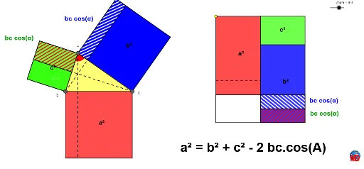
This example visually demonstrates the Law of Cosines in arbitrary triangles through dynamic geometry. It involves core concepts like the Law of Cosines, triangle side-angle relationships, and vector operations. Construction highlights include using GeoGebra commands such as Line, Polygon, OrthogonalLine, Intersect, Segment, Angle, Ray, Rotate, Circle, and Midpoint to build triangles and auxiliary lines, dynamically adjusting sides and angles to illustrate the theorem's generality. Suitable for high school mathematics instruction and geometric theorem exploration.
GeoGebra Commands & Parameters
Line(B, A) → dPolygon(B, A, 4) → poly4, r, s, t, a_1, K, LLine(L, K) → b_1Line(C, A) → eOrthogonalLine(B, e) → gIntersect(e, g) → FPolygon(A, C, 4) → poly3, m, n, p, q, I, JLine(I, J) → c_1Intersect(g, c_1) → NPolygon(A, F, N, J) → poly6, a_3, f_1, n_1, j_1Polygon(C, I, N, F) → poly10, c_3, i_1, n_2, f_2OrthogonalLine(C, d) → fIntersect(d, f) → EIntersect(f, b_1) → MPolygon(A, E, M, K) → poly5, a_2, e_1, m_1, k_1Polygon(B, E, M, L) → poly9, b_3, e_2, m_2, l_1Polygon(C, B, 4) → poly2, i, j, k, l, G, HLine(V, K_1) → t_2Line(Z, D_1) → e_3Intersect(t_2, e_3) → L_1Polygon(A, B, C) → poly1, c, a, bOrthogonalLine(A, a) → hIntersect(h, a) → DIntersect(h, k) → OPolygon(D, C, H, O) → poly7, d_1, c_2, h_1, o_2Polygon(D, O, G, B) → poly8, d_2, o_1, g_1, b_2Segment(A, D) → p_1Segment(C, E) → q_1Segment(B, F) → r_1Angle(B, A, C) → αSegment(A, E) → s_1Segment(A, F) → t_1Ray(B, C) → g_2Ray(C, B) → h_2Rotate(C, (-((180° - setalpha) / 2)), C) → C'Rotate(B, (-((180° - (2 * setalpha)) / 2)), C) → B'Ray(C', B') → i_2Rotate(B, (180° - (2 * setalpha)) / 2, B) → B'_1Rotate(C, (180° - (2 * setalpha)) / 2, B) → C'_1Ray(B'_1, C'_1) → j_2Intersect(i_2, j_2) → PCircle(P, C) → k_2Ray(D, A) → l_2Intersect(k_2, l_2) → Q,Midpoint(B, C) → RCircle(R, C) → p_2Intersect(p_2, l_2) → S, C_1Polygon(T, J_1, I_1, H_1) → poly16, t_3, j_3, i_4, h_4Polygon(H_1, I_1, K_1, V) → poly11, h_3, i_3, k_3, vLine(W, F_1) → l_3Intersect(l_3, v) → M_1Polygon(H_1, I_1, W, M_1) → poly15, h_5, i_5, w, m_3Polygon(H_1, V, K_1, I_1) → poly17, n_3, p_3, q_3, r_3Polygon(H_1, I_1, W, M_1) → poly18, h_6, i_6, w_1, m_4Polygon(M_1, W, K_1, V) → poly19, m_5, w_2, k_4, v_1Polygon(W, F_1, L_1, K_1) → poly20, q_2, r_2, s_2, f_3Polygon(U, Z, B_1, A_1) → poly12, u_1, z, b_4, a_4Polygon(A_1, B_1, N_1, G_1) → poly13, d_3, s_3, c_4, e_4Polygon(K_1, G_1, N_1, D_1) → poly14, k_5, g_3, n_4, d_4Line(G_1, N_1) → f_4Line(T, V) → g_4Intersect(f_4, g_4) → O_1Segment(M_1, O_1) → j_4Segment(O_1, G_1) → l_4Midpoint(B, H) → Q_1Midpoint(J, C) → R_1Midpoint(K, B) → S_1Midpoint(A_1, Z) → T_1Midpoint(t_1) → U_1Midpoint(F_1, K_1) → V_1Midpoint(D_1, G_1) → W_1Midpoint(J, F) → Z_1Midpoint(K, E) → A_2Midpoint(T, W) → P_1Segment(H_1, I_1) → p_4Polygon(L, K, A, B) → poly21, l_5, k_6, a_5, b_5Midpoint(B_1, G_1) → C_2Polygon(J, I, C, A) → poly22, j_5, i_7, c_5, a_6Midpoint(F_1, D_1) → D_2Midpoint(D_1, N_1) → E_2
AI Drawing Prompt Reference
Draw an arbitrary triangle to visually demonstrate the Law of Cosines. Include the triangle's three sides and angles, with auxiliary lines highlighting the key relationships in the theorem. Use perpendicular lines, intersection points, and rotation to construct auxiliary shapes, showing the theorem's generality as sides and angles change. The final image should clearly illustrate the connection between the triangle's parts and the Law of Cosines, suitable for high school mathematics instruction and geometric theorem exploration.
The prompt above was compiled from the original drawing commands and is for reference only.