
Vertical Dilations: Compression Patterns When 0<a<1
Loading the math board and drawing, please wait…
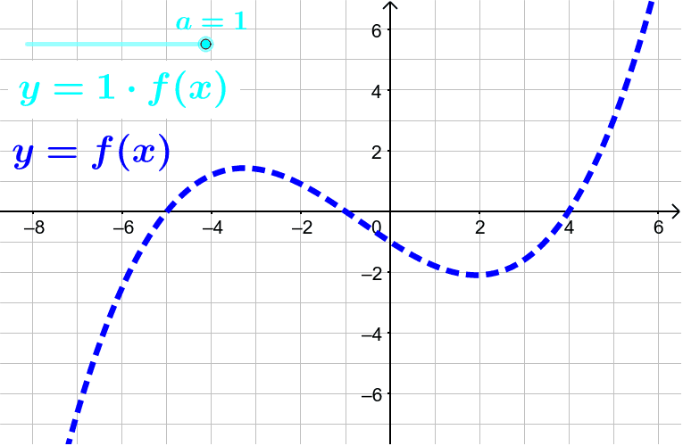
This example demonstrates how function graphs compress vertically when the dilation coefficient a is between 0 and 1. By using a slider to control parameter a, users can observe how function f(x) transforms into g(x)=a·f(x) through vertical dilation. The construction uses the Sequence command to generate transformation sequences, with slider object a controlling the dilation factor, visualizing the comparison between functions f and g. Ideal for secondary school mathematics courses teaching function transformations, and for exploring the relationship between dilation factors and graph shapes, developing students' ability to connect algebra and geometry.
GeoGebra Commands & Parameters
Sequence(Segment[(i, g(i)), (i, 0)], i, -6, 6, 1.5) → list1
AI Drawing Prompt Reference
Draw the graph of a base function f(x) together with its vertically compressed version g(x)=a·f(x), where a is a slider ranging from 0 to 1; at x-values from -6 to 6 in steps of 1.5, add vertical segments from the x-axis up to the curve of g(x) to illustrate the compression effect. The segments are drawn at each sampled x-coordinate, showing how the height of g(x) shrinks as a decreases.
The prompt above was compiled from the original drawing commands and is for reference only.