
Upper and Lower Sum of a Function
Loading the math board and drawing, please wait…
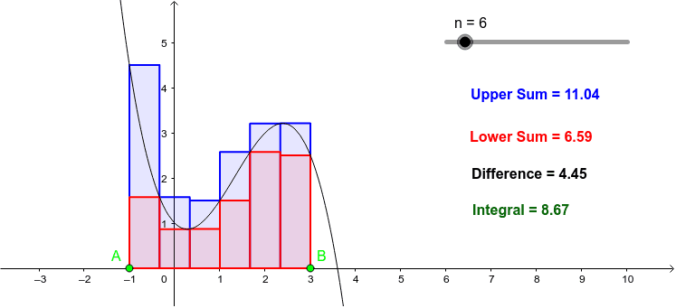
This example visualizes the upper and lower sums of a cubic polynomial to help understand the basic concept of integration. It involves key mathematical concepts such as functions, integration, and interval partitioning. The commands used include Point, UpperSum, LowerSum, and Integral. By adjusting the number of intervals n, one can observe and understand the changes in upper and lower sums. Suitable for high school mathematics education and learning.
GeoGebra Commands & Parameters
Point(xAxis) → APoint(xAxis) → BUpperSum(f, x(A), x(B), n) → uppersumLowerSum(f, x(A), x(B), n) → lowersumIntegral(f, x(A), x(B)) → F
AI Drawing Prompt Reference
Draw a cubic function curve on a coordinate plane. Place two points on the x-axis to define an interval. Between these endpoints, construct a series of equal-width rectangles that approximate the area under the curve from above (upper sum) and from below (lower sum), using distinct colors for each set. Also fill the exact area under the curve between the endpoints with a semi-transparent shade. The number of rectangles can be adjusted to show how the upper and lower sums converge to the exact integral.
The prompt above was compiled from the original drawing commands and is for reference only.