Upper and Lower Riemann Sums – Visualizing Definite Integral Approximation

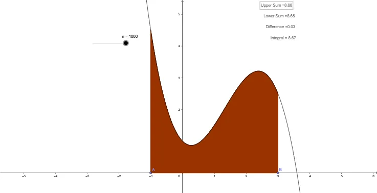
This example demonstrates how to construct upper and lower Riemann sums for a function f over an interval [a,b] and compare them with the definite integral using GeoGebra. The commands UpperSum, LowerSum, and Integral are employed, together with objects such as f, A, B, n, a, b, and sliders for dynamic exploration. Users can see how the upper and lower sums converge to the exact integral as the number of subintervals n increases. Core concepts include Riemann sums, upper and lower bounds, approximation of definite integrals, and the limit definition of integration. It is suitable for high‑school or first‑year university calculus courses.