
Riemann Sum Demo (Left, Right, Midpoint)
Loading the math board and drawing, please wait…
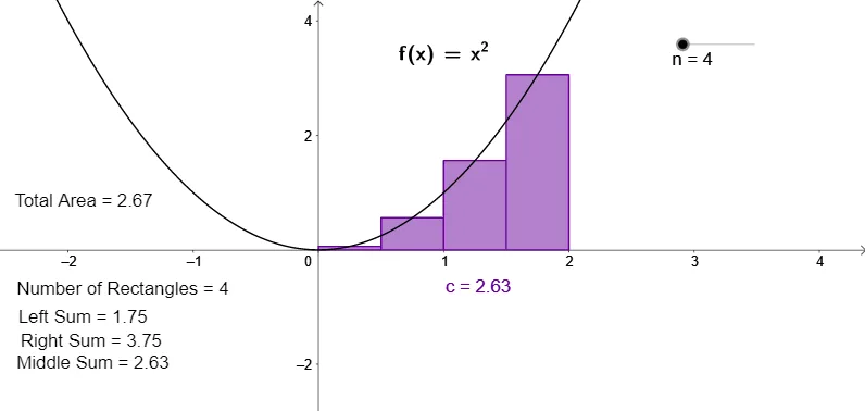
① This example demonstrates how left‑endpoint, right‑endpoint, and midpoint Riemann sums approximate the area under a curve for a definite integral. ② Core mathematical concepts include the definite integral, Riemann sums, the limit process, and error analysis of numerical integration. ③ Construction highlights: GeoGebra commands Intersect, Point, LeftSum, UpperSum, RectangleSum, LaTeX, Integral and objects f, n, A, B, a, b, c, text1‑text6, d are used to build the function graph, partition rectangles, dynamic sliders, and annotation texts. ④ Suitable for high‑school calculus electives, introductory university calculus courses, and self‑study; it works well as a classroom interactive tool or homework aid.
GeoGebra Commands & Parameters
Intersect(f, xAxis, 1) → APoint(xAxis) → BLeftSum(f, x(A), x(B), n) → aUpperSum(f, x(A), x(B), n) → bRectangleSum(f, x(A), x(B), n, 0.5) → cLaTeX(f, true, true) → text5Integral(f, 0, 2) → d
AI Drawing Prompt Reference
Draw a function graph with its x-axis below. Demonstrate three methods to approximate the area under the curve from 0 to 2: left-endpoint, right-endpoint, and midpoint Riemann sums using rectangles. Use dynamic sliders to control the number of rectangles for each method. Annotate the function expression and integral result, highlighting this as a demonstration of definite integrals, Riemann sums, the limit process, and error analysis in numerical integration.
The prompt above was compiled from the original drawing commands and is for reference only.