
Unit Circle and Sine Curve: Dynamic Visualization
Loading the math board and drawing, please wait…
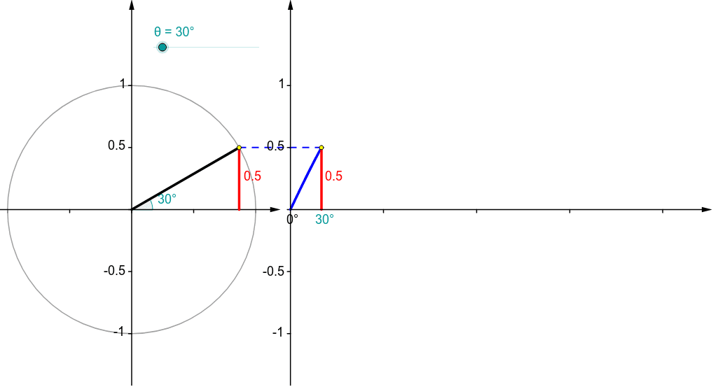
This GeoGebra example dynamically demonstrates the correspondence between a point rotating on the unit circle and the graph of the sine function, showing how angle changes map to points on the sine curve. Core mathematical concepts include trigonometric definitions, the unit circle, radian measure, periodicity, and function graphing. Construction highlights: using commands such as Point, Rotate, Angle, Function, Segment, Circle, Vector, and Sequence, the applet creates a moving point P on the unit circle with angle θ, plots the sine function f, and constructs auxiliary segments, vectors, and point lists. A slider controls the angle for real-time interaction. Suitable for high school trigonometry, pre-calculus review, and teacher-made interactive lessons, this helps students grasp the geometric origin and periodic nature of the sine function.
GeoGebra Commands & Parameters
Point(Ray[(0, 0), (-1, 0)]) → BRotate(A, θ, B) → PRotate(A, θ, B) → A'Angle(A, B, A') → αRotate(A, θ, B) → A'_1Angle(A, B, A'_1) → βFunction(sin(120° * x), 0, x(Q)) → fSegment(Q, (x(Q), 0)) → eCircle(B, A) → cSegment(B, P) → aVector((x(B), y(Corner[1])), (x(B), y(Corner[4]))) → uVector((0, y(Corner[1])), (0, y(Corner[4]))) → wVector((0, 0), (x(Corner[2]), 0)) → zSequence(Segment[(0.75 * i, 0), (0.75 * i, -0.025)], i, 1, 4) → list1Segment(P, (x(P), 0)) → bVector(B - (1.2, 0), B + (1.2, 0)) → vSequence(Segment[(0, 0.5 * i - 1), (-0.025, 0.5 * i - 1)], i, 0, 4) → list2Sequence(Segment[(x(B), 0.5 * i - 1), (x(B) - 0.025, 0.5 * i - 1)], i, 0, 4) → list3Segment(P, Q) → dSequence(Segment[B + (0.5 * i - 1, 0), B + (0.5 * i - 1, -0.025)], i, 0, 4) → list4Point(Ray[(0, 0), (-1, 0)]) → B_1Rotate(A_1, θ, B_1) → P_1Rotate(A_1, θ, B_1) → A'_2Rotate(A_1, θ, B_1) → A'_3Circle(B_1, A_1) → c_1Segment(B_1, P_1) → a_1
AI Drawing Prompt Reference
Draw a unit circle centered at the origin with radius one. Place a rotating point on the circle, connected to the center by a radius, and display the corresponding angle. Drop a perpendicular from this point to the x-axis, marking the foot. To the right, plot the sine curve with the horizontal axis as angle in radians and vertical axis as sine value. Connect the y-coordinate of the circle point to the corresponding point on the curve with a dashed line to show the mapping. Add a slider to control the angle, and include tick marks and coordinate axes.
The prompt above was compiled from the original drawing commands and is for reference only.