
Understand Cubic Graphs by Factorization (No Calculus)
Loading the math board and drawing, please wait…
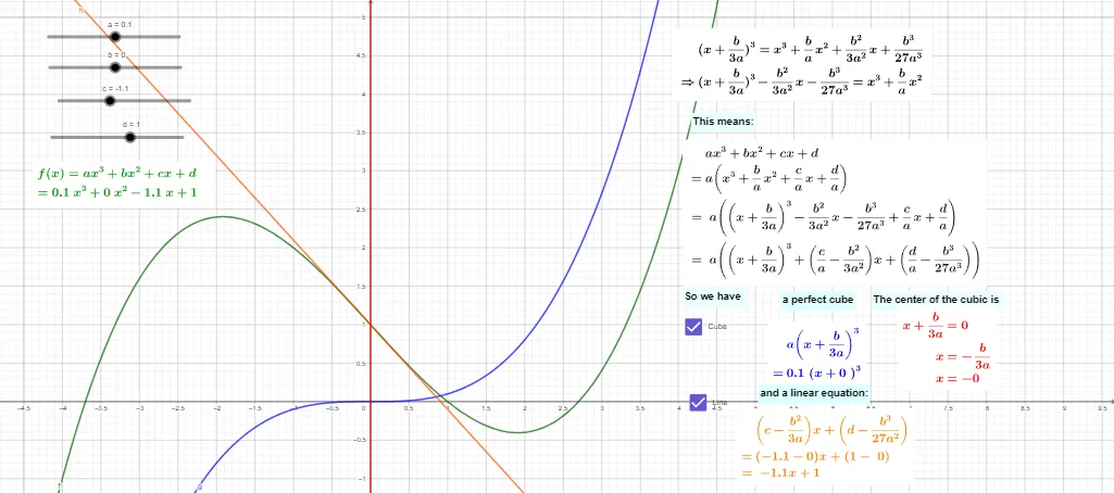
This GeoGebra example demonstrates how to understand a cubic equation’s graph by breaking the polynomial into factors, connecting algebraic structure to geometric features such as intercepts/zeros on the x-axis. The key mathematical ideas are cubic polynomials, factorization of expressions, roots, and graph interpretation of polynomial functions (including the role of straight lines like the x-axis in locating intersections). Construction is guided by the provided GeoGebra setup: it uses the command “Factors” to obtain the factor form of the algebraic object, and it creates/manages multiple intermediate variables (e.g., a, b, c, d, e, f, g, h, i, j, k, l) along with equation/expression objects (such as eq1). The example also relies on text objects (text1–text11) to label steps and results, making the link between the factorization and the resulting graph features explicit. Suitable for middle to high school and early precalculus learners, as well as for classroom demonstrations focused on algebraic reasoning instead of calculus.
GeoGebra Commands & Parameters
Factors(f) → m1
AI Drawing Prompt Reference
On a single coordinate plane, create a visual explanation of a cubic polynomial’s graph by first expressing the given cubic as a factorized product. Use the factorization to identify the polynomial’s zeros/roots and clearly connect them to where the curve intersects the x-axis. Then present a guided sequence of labeled step results (as text) that link each algebraic factor to its geometric meaning—how the located roots determine the intercepts and the resulting behavior of the cubic curve. Finally show the resulting cubic graph for interpretation, emphasizing the algebra-to-geometry connection without relying on calculus.
The prompt above was compiled from the original drawing commands and is for reference only.