
Try to Graph the Derivative Function by Marc Renault
Loading the math board and drawing, please wait…
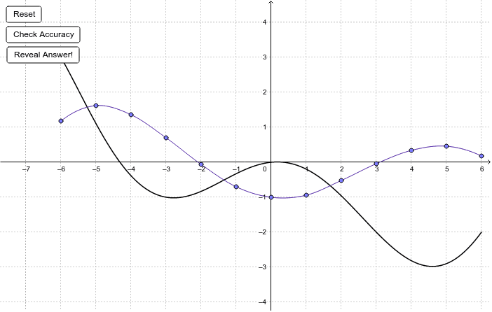
This example demonstrates how to infer and graph the derivative function by analyzing the original function's graph. Key math concepts include the geometric meaning of derivatives, function graph characteristics, and linear fitting. GeoGebra commands/objects used in construction are Sequence, Corner, FitPoly, Function, Segment, and Point. Suitable for high school students learning introductory calculus to understand the relationship between derivatives and original function graphs.
GeoGebra Commands & Parameters
Sequence((i, Random[-2, 3] + (0 * dummy)), i, -12, 12, 3) → fPointListCorner(1) → panelPt1Corner(4) → panelPt4FitPoly(fPointList, Length[fPointList] - 1) → fFunction(f, -6, 6) → fResFunction(g, -6, 6) → gResSegment((-6, -3.5), (-6, 4.5)) → segASegment((-5, -3.5), (-5, 4.5)) → segBSegment((-4, -3.5), (-4, 4.5)) → segCSegment((-3, -3.5), (-3, 4.5)) → segDSegment((-2, -3.5), (-2, 4.5)) → segESegment((-1, -3.5), (-1, 4.5)) → segFSegment((0, -3.5), (0, 4.5)) → segGSegment((1, -3.5), (1, 4.5)) → segHSegment((2, -3.5), (2, 4.5)) → segISegment((3, -3.5), (3, 4.5)) → segJSegment((4, -3.5), (4, 4.5)) → segKSegment((5, -3.5), (5, 4.5)) → segLSegment((6, -3.5), (6, 4.5)) → segMPoint(segA) → APoint(segB) → BPoint(segC) → CPoint(segD) → DPoint(segE) → EPoint(segF) → FPoint(segG) → GPoint(segH) → HPoint(segI) → IPoint(segJ) → JPoint(segK) → KPoint(segL) → LPoint(segM) → MFitPoly({A, B, C}, 2) → parABCFitPoly({C, D, E}, 2) → parCDEFitPoly({E, F, G}, 2) → parEFGFitPoly({G, H, I}, 2) → parGHIFitPoly({I, J, K}, 2) → parIJKFitPoly({K, L, M}, 2) → parKLMFitPoly({B, C, D}, 2) → parBCDFitPoly({D, E, F}, 2) → parDEFFitPoly({F, G, H}, 2) → parFGHFitPoly({H, I, J}, 2) → parHIJFitPoly({J, K, L}, 2) → parJKLFunction(parABC, x(A), x(B)) → conABFunction((parABC(x) * (1 - (x + 5))) + (parBCD(x) * (x + 5)), -5, -4) → conBCFunction((parBCD(x) * (1 - (x + 4))) + (parCDE(x) * (x + 4)), -4, -3) → conCDFunction((parCDE(x) * (1 - (x + 3))) + (parDEF(x) * (x + 3)), -3, -2) → conDEFunction((parDEF(x) * (1 - (x + 2))) + (parEFG(x) * (x + 2)), -2, -1) → conEFFunction((parEFG(x) * (1 - (x + 1))) + (parFGH(x) * (x + 1)), -1, 0) → conFGFunction((parFGH(x) * (1 - (x + 0))) + (parGHI(x) * (x + 0)), 0, 1) → conGHFunction((parGHI(x) * (1 - (x - 1))) + (parHIJ(x) * (x - 1)), 1, 2) → conHIFunction((parHIJ(x) * (1 - (x - 2))) + (parIJK(x) * (x - 2)), 2, 3) → conIJFunction((parIJK(x) * (1 - (x - 3))) + (parJKL(x) * (x - 3)), 3, 4) → conJKFunction((parJKL(x) * (1 - (x - 4))) + (parKLM(x) * (x - 4)), 4, 5) → conKLFunction(parKLM, 5, 6) → conLM
AI Drawing Prompt Reference
Draw the graph of a function and its derivative. First, randomly generate the graph of a function, then fit a polynomial to the derivative based on the function's characteristics. Draw a rectangular area on the y-axis, and use the fitted polynomials to connect adjacent inflection points, constructing the derivative function's graph. Finally, use these polynomial functions to draw the continuous derivative function.
The prompt above was compiled from the original drawing commands and is for reference only.