
Try to Graph the Derivative Function by drdrew42
Loading the math board and drawing, please wait…
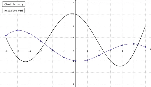
① This example demonstrates an interactive activity where users attempt to sketch the derivative function of a given original function, with GeoGebra providing visual feedback. ② The core mathematical concept is the geometric interpretation of the derivative: the derivative function represents the slope of the tangent line at each point of the original function. Users infer the sign and zeros of the derivative by analyzing where the original function increases, decreases, or has extrema. ③ Construction details: Based on the summary, the construction uses commands such as FitPoly (to generate a polynomial approximation of the original function), Function (to define functions), Segment and Point (to create auxiliary segments and points), and Corner/panelWidth (to manage the display panel). Objects include multiple points (S, T, U, V, W, X, Y, Z, R) and segments (segA through segM), as well as result objects fRes and gRes, likely for comparing the user's sketch with the actual derivative. ④ This is suitable for high school or introductory college calculus students, serving as an interactive exercise or teacher demonstration to build intuition about derivatives.
GeoGebra Commands & Parameters
Corner(1) → panelPt1Corner(4) → panelPt4FitPoly({R, S, T, U, V, W, X, Y, Z}, 8) → fFunction(f, -6, 6) → fResFunction(g, -6, 6) → gResSegment((-6, -3.5), (-6, 4.5)) → segASegment((-5, -3.5), (-5, 4.5)) → segBSegment((-4, -3.5), (-4, 4.5)) → segCSegment((-3, -3.5), (-3, 4.5)) → segDSegment((-2, -3.5), (-2, 4.5)) → segESegment((-1, -3.5), (-1, 4.5)) → segFSegment((0, -3.5), (0, 4.5)) → segGSegment((1, -3.5), (1, 4.5)) → segHSegment((2, -3.5), (2, 4.5)) → segISegment((3, -3.5), (3, 4.5)) → segJSegment((4, -3.5), (4, 4.5)) → segKSegment((5, -3.5), (5, 4.5)) → segLSegment((6, -3.5), (6, 4.5)) → segMPoint(segA) → APoint(segB) → BPoint(segC) → CPoint(segD) → DPoint(segE) → EPoint(segF) → FPoint(segG) → GPoint(segH) → HPoint(segI) → IPoint(segJ) → JPoint(segK) → KPoint(segL) → LPoint(segM) → MFitPoly({A, B, C}, 2) → parABCFitPoly({C, D, E}, 2) → parCDEFitPoly({E, F, G}, 2) → parEFGFitPoly({G, H, I}, 2) → parGHIFitPoly({I, J, K}, 2) → parIJKFitPoly({K, L, M}, 2) → parKLMFitPoly({B, C, D}, 2) → parBCDFitPoly({D, E, F}, 2) → parDEFFitPoly({F, G, H}, 2) → parFGHFitPoly({H, I, J}, 2) → parHIJFitPoly({J, K, L}, 2) → parJKLFunction(parABC, x(A), x(B)) → conABFunction((parABC(x) * (1 - (x + 5))) + (parBCD(x) * (x + 5)), -5, -4) → conBCFunction((parBCD(x) * (1 - (x + 4))) + (parCDE(x) * (x + 4)), -4, -3) → conCDFunction((parCDE(x) * (1 - (x + 3))) + (parDEF(x) * (x + 3)), -3, -2) → conDEFunction((parDEF(x) * (1 - (x + 2))) + (parEFG(x) * (x + 2)), -2, -1) → conEFFunction((parEFG(x) * (1 - (x + 1))) + (parFGH(x) * (x + 1)), -1, 0) → conFGFunction((parFGH(x) * (1 - (x + 0))) + (parGHI(x) * (x + 0)), 0, 1) → conGHFunction((parGHI(x) * (1 - (x - 1))) + (parHIJ(x) * (x - 1)), 1, 2) → conHIFunction((parHIJ(x) * (1 - (x - 2))) + (parIJK(x) * (x - 2)), 2, 3) → conIJFunction((parIJK(x) * (1 - (x - 3))) + (parJKL(x) * (x - 3)), 3, 4) → conJKFunction((parJKL(x) * (1 - (x - 4))) + (parKLM(x) * (x - 4)), 4, 5) → conKLFunction(parKLM, 5, 6) → conLM
AI Drawing Prompt Reference
Draw a coordinate plane with x-axis from -6 to 6 and y-axis from -3.5 to 4.5. Place vertical dashed lines at each integer x-coordinate from -6 to 6, extending from the bottom to the top of the y-axis. On each vertical line, put a movable point, making thirteen points in total. Connect these points with a smooth curve to form an eighth-degree polynomial. Then, for every three adjacent points, fit a quadratic parabola, and smoothly join these parabolas into a continuous piecewise curve as an approximation of the original function. Finally, in the same coordinate range, draw another curve representing the derivative of the original function, whose shape reflects where the original increases or decreases.
The prompt above was compiled from the original drawing commands and is for reference only.