
Try to Graph the Derivative Function
Loading the math board and drawing, please wait…
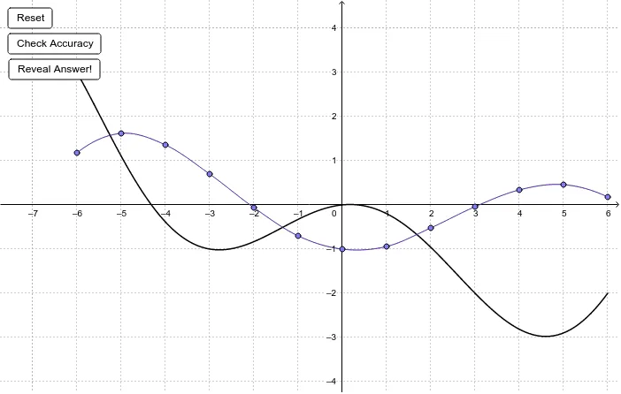
This example demonstrates how to graph the derivative function based on the given function graph. Key mathematical concepts include derivatives. Using GeoGebra commands such as Sequence, Function, and Segment, the derivative function graph can be constructed. Suitable for high school mathematics education and learning calculus concepts.
GeoGebra Commands & Parameters
Sequence((i, Random[-2, 3] + (0 * dummy)), i, -12, 12, 3) → fPointListCorner(1) → panelPt1Corner(4) → panelPt4FitPoly(fPointList, Length[fPointList] - 1) → fFunction(f, -6, 6) → fResFunction(g, -6, 6) → gResSegment((-6, -3.5), (-6, 4.5)) → segASegment((-5, -3.5), (-5, 4.5)) → segBSegment((-4, -3.5), (-4, 4.5)) → segCSegment((-3, -3.5), (-3, 4.5)) → segDSegment((-2, -3.5), (-2, 4.5)) → segESegment((-1, -3.5), (-1, 4.5)) → segFSegment((0, -3.5), (0, 4.5)) → segGSegment((1, -3.5), (1, 4.5)) → segHSegment((2, -3.5), (2, 4.5)) → segISegment((3, -3.5), (3, 4.5)) → segJSegment((4, -3.5), (4, 4.5)) → segKSegment((5, -3.5), (5, 4.5)) → segLSegment((6, -3.5), (6, 4.5)) → segMPoint(segA) → APoint(segB) → BPoint(segC) → CPoint(segD) → DPoint(segE) → EPoint(segF) → FPoint(segG) → GPoint(segH) → HPoint(segI) → IPoint(segJ) → JPoint(segK) → KPoint(segL) → LPoint(segM) → MFitPoly({A, B, C}, 2) → parABCFitPoly({C, D, E}, 2) → parCDEFitPoly({E, F, G}, 2) → parEFGFitPoly({G, H, I}, 2) → parGHIFitPoly({I, J, K}, 2) → parIJKFitPoly({K, L, M}, 2) → parKLMFitPoly({B, C, D}, 2) → parBCDFitPoly({D, E, F}, 2) → parDEFFitPoly({F, G, H}, 2) → parFGHFitPoly({H, I, J}, 2) → parHIJFitPoly({J, K, L}, 2) → parJKLFunction(parABC, x(A), x(B)) → conABFunction((parABC(x) * (1 - (x + 5))) + (parBCD(x) * (x + 5)), -5, -4) → conBCFunction((parBCD(x) * (1 - (x + 4))) + (parCDE(x) * (x + 4)), -4, -3) → conCDFunction((parCDE(x) * (1 - (x + 3))) + (parDEF(x) * (x + 3)), -3, -2) → conDEFunction((parDEF(x) * (1 - (x + 2))) + (parEFG(x) * (x + 2)), -2, -1) → conEFFunction((parEFG(x) * (1 - (x + 1))) + (parFGH(x) * (x + 1)), -1, 0) → conFGFunction((parFGH(x) * (1 - (x + 0))) + (parGHI(x) * (x + 0)), 0, 1) → conGHFunction((parGHI(x) * (1 - (x - 1))) + (parHIJ(x) * (x - 1)), 1, 2) → conHIFunction((parHIJ(x) * (1 - (x - 2))) + (parIJK(x) * (x - 2)), 2, 3) → conIJFunction((parIJK(x) * (1 - (x - 3))) + (parJKL(x) * (x - 3)), 3, 4) → conJKFunction((parJKL(x) * (1 - (x - 4))) + (parKLM(x) * (x - 4)), 4, 5) → conKLFunction(parKLM, 5, 6) → conLM
AI Drawing Prompt Reference
Draw a function graph and its derivative graph. First, generate a random function graph. Then, based on this graph, create a derivative function graph. Next, draw a series of vertical segments, with each segment's length representing the function value and its position corresponding to integer points on the x-axis. Finally, fit polynomials to connect the vertices of adjacent segments, approximating the derivative function's curve.
The prompt above was compiled from the original drawing commands and is for reference only.