
Trigonometric & Linear Transformations Demo
Loading the math board and drawing, please wait…
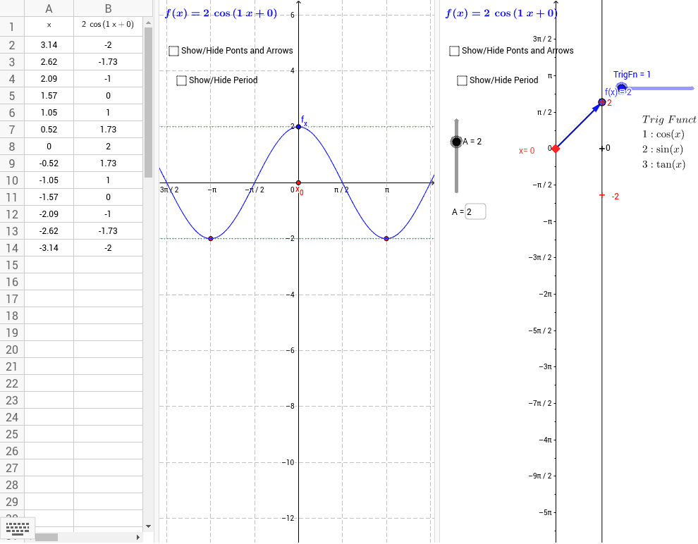
This example demonstrates the linear transformations of trigonometric functions and their loci in a coordinate plane. It involves core concepts like trigonometry, linear functions, derivatives, and transformations. Constructed using GeoGebra commands like Point, Vector, Segment, Sequence, Textfield, Derivative, Zip, it is ideal for high school and above students to explore function transformations and calculus applications.
GeoGebra Commands & Parameters
Element(TrigL, TrigFn) → fPoint(yAxis) → aVector(a, f_a) → uSegment(C_1, D) → eVector(E, F) → vSequence((k, f(k)), k, C - π, C + π, 0.5235987755982988) → list1Sequence(Vector[(0, k), (2, f(k))], k, C - π, C + π, 0.5235987755982988) → list2Sequence(Segment[(i, f(i)), ((2 * C) - i, f((2 * C) - i))], i, C - π, C, 0.5235987755982988) → list3Vector(G, H) → wSegment(f_x, J) → jSequence(Segment[(i, f(i)), (π - i, f(π - i))], i, 0, 3.141592653589793, 0.5235987755982988) → suplTextfield(B) → inputBox1Textfield(C) → InputBox1Derivative(f) → f'Vector(f_a, (2, y(f_a) + f'(y(a)))) → hSequence(-5, 5) → nlistZip(((1 / B * ((2 * k) + 1)) * π / 2) - C / B, k, nlist) → xtrslistZip((z, f(z)), z, xtrslist) → xtrsptsZip(((1 / B * k) * π) - C / B, k, nlist) → xrtclistZip((z, f(z)), z, xrtclist) → xtrcptsTextfield(A) → InputBox2Segment(a, Q) → lSegment(a, P) → mVector(P, f_a) → nVector(Q, f_a) → pSegment(f_x, M) → sSegment(f_x, R) → q
AI Drawing Prompt Reference
Draw a trigonometric function and its linear transformation locus in a coordinate plane, showing the original function, vertical translation vector, symmetric line segments, and transformed function images, with the origin, symmetry axis, and transformation vectors labeled, and finally plot multiple linearly transformed function images with an input box for interaction.
The prompt above was compiled from the original drawing commands and is for reference only.