Trigonometric Equation All-Solutions Solver with Complex and Vector Dynamics

Loading the math board and drawing, please wait…

2017-01-29 01:28

In collections Mapping Diagrams: From AB to C&DE, Resource

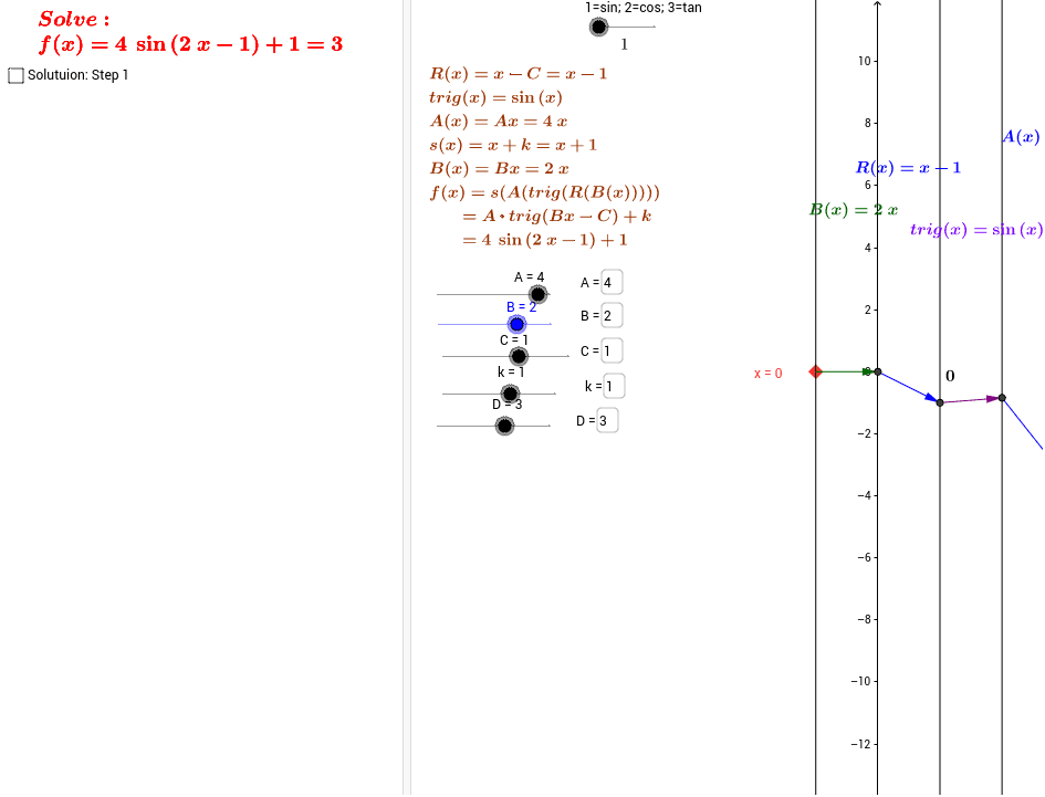
① This GeoGebra example presents an interactive solver for trigonometric equations, dynamically illustrating the complete set of solutions (All Solve Eqn.3) under complex parameters and vector translations. ② Core mathematical concepts include periodicity of trigonometric functions, general solution formulas, root distribution in the complex plane, vector translation transformations, and the role of derivatives in equation analysis. ③ Construction highlights: using commands like Element, Textfield, Point, and Vector to create input boxes and dynamic points; objects such as D_n, b, trl, B, mf, fnum, trig, C, R, k, s, A, i, K control equation parameters; complex objects and vector translations (atrl, atrig) enable dynamic visualization of solutions; text displays (text1, text6, text8) and sliders provide interactive control. ④ Suitable for high school to undergraduate students studying trigonometry, complex numbers, and transformations, as well as for teachers demonstrating general solutions and geometric interpretations in class.

GeoGebra Commands & Parameters

Element(trl, fnum) → trig
Element(atrl, fnum) → atrig
Element(atrl2, fnum) → atrig2
Textfield(B) → inputBox1
Textfield(s) → inputBoxf
Point(b) → A_x
Vector(K, s_{inv}D) → w
Vector(s_{inv}D, m_{invSinvD}) → z
Vector(m_{invSinvD}, q_{inv+}) → d
Vector(q_{inv+}, I) → h_1
Textfield(C) → inputBox2
Textfield(k) → inputBox3
Textfield(A) → inputBox4
Textfield(B) → inputBox5
Textfield(s) → inputBox6
Vector(m_{invSinvD}, P_2) → u
Vector(P_2, J) → j
Vector(I, E) → v
Vector(J, D) → c
Textfield(B) → inputBox7
Vector(A_x, F) → m
Vector(F, G) → n
Vector(G, H) → p
Vector(H, L) → q
Vector(L, M) → r
Textfield(D_n) → inputBox8