
Geometric Interpretation of Discrete Fourier Transform
Loading the math board and drawing, please wait…
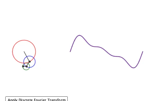
This example demonstrates the principle of the Discrete Fourier Transform through geometric figures. It involves complex numbers, vectors, and transformations. Using GeoGebra commands such as Circle, Vector, If, Segment, and PolyLine, users can visually understand the process of the Discrete Fourier Transform. Suitable for university mathematics and signal processing courses.
GeoGebra Commands & Parameters
Circle(A2, R3) → c3Vector(A1, P1) → v1Vector(A2, P1) → v2Vector(A3, P1) → v3If(n ≟ 1, v1, Vector[If[n ≟ 2, v2, v3]]) → vCircle((-4, -2.5), R1) → d1Circle((-4, -4.5), R2) → d2Circle((-4, -6.5), R3) → d3Segment(Center[d1], B1) → b1Segment(Center[d2], B2) → b2Segment(Center[d3], B3) → b3Vector(B1, (t, f1(t))) → u1Vector(B2, (t, f2(t))) → u2Vector(B3, (t, f3(t))) → u3Circle((x(A1), y(A1)), R2) → c2Circle((-4, -4.5), R1) → c1PolyLine((-4, -4.5), A1, A2, A3) → pVector((-4, -4.5), ((-4, -4.5) * (1 - sep)) + (sep * A1)) → vs2Translate(d2, vs2) → c20Vector((-4, -6.5), ((-4, -6.5) * (1 - sep)) + (sep * A2)) → vs3Translate(d3, vs3) → c30Vector((-4, -2.5), (-4, (-4.5 * sep) + ((1 - sep) * (-2.5)))) → vs1Vector((-4, -2.5), (-4, (-4.5 * sep) + ((1 - sep) * (-2.5)))) → vs10Translate(f1, vs10) → ff1Vector((-4, -6.5), (-4, (-4.5 * sep) + ((1 - sep) * (-6.5)))) → vs30Translate(d1, vs1) → c10Translate(f3, vs30) → ff3