
Traffic Acceleration Simulation: Quadratic Functions & Motion Graphs
Loading the math board and drawing, please wait…
In collections
Traffic
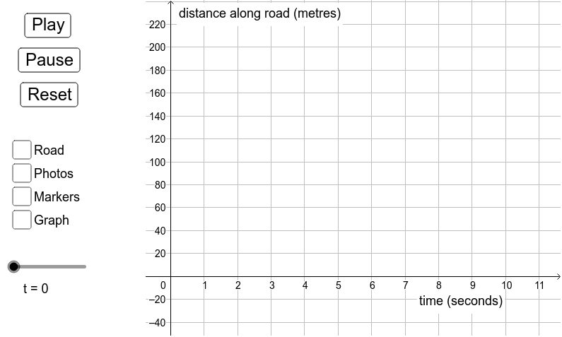
This example demonstrates traffic acceleration dynamics using mathematical modeling. It covers core concepts like quadratic functions, curve sketching, and parametric motion. Construction utilizes GeoGebra commands such as Sequence and Segment to render road elements and vehicle trajectories controlled by variables t, a, b, c, d. Ideal for high school students studying calculus or algebra to visualize acceleration rates and function behavior in real-world contexts.
GeoGebra Commands & Parameters
Sequence((n, g(n)), n, 0, t_1) → list2Segment((-1.9, 0), (-1.1, 0)) → road_0Sequence(i - 0.4 < x < i + 0.4, i, 0, t_1) → photo_{road}Sequence(x = i - 0.4, i, 0, t_1) → left_{road}Sequence(x = i + 0.4, i, 0, t_1) → right_{road}Sequence(x = i, i, 0, t_1) → mid_{road}Sequence(Translate[car_p, Vector[(0, g(0)), (i - g_y(i), g(i))]], i, 0, t_1) → photo_rSegment((-1.9, 200), (-1.1, 200)) → road_{200}
AI Drawing Prompt Reference
Draw a traffic acceleration simulation with a road and vehicle trajectories. The road is divided into segments from 0 to t1, with dashed lines every 0.4 units. Vehicle trajectories are controlled by function g(t) as t varies from 0 to t1. There are dashed lines on both sides of the road and a solid line in the middle. Vehicles move along the road with accelerating motion, forming parabolic trajectories.
The prompt above was compiled from the original drawing commands and is for reference only.