
Nautilus Logarithmic Spiral Parametric Construction
Loading the math board and drawing, please wait…
In collections
geometriadinamica.es
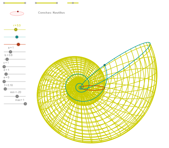
This GeoGebra example demonstrates how to construct a nautilus (sea shell) logarithmic spiral using parametric equations. The core mathematical concept is the equiangular (logarithmic) spiral, described by x=a*e^(b*θ)*cos(θ), y=a*e^(b*θ)*sin(θ) in Cartesian coordinates. Key construction commands include: CurveCartesian for plotting the parametric curve, Sequence for generating θ values, Ellipse and Circle for auxiliary geometric structures, Point for placing key points, and Angle for measuring spiral angles. This example is suitable for high school mathematics (coordinate geometry, parametric equations) and college calculus (curve theory, polar coordinates), serving as an excellent case study for mathematical modeling of natural phenomena.
GeoGebra Commands & Parameters
Segment(Q3, Q4) → p2Point(p2) → P3Segment(P3, Q4) → p4Point(p4) → P4Segment(Q1, Q2) → p1Point(p1) → P1Segment(P1, Q2) → p3Point(p3) → P2OrthogonalLine(C, yAxis) → zz1Circle(C, 0.62) → zz0Intersect(zz0, zz1, 1) → ZZ1Intersect(zz0, zz1, 2) → ZZ2Ellipse(ZZ1, ZZ2, 0.65) → zElipse1Intersect(zElipse1, zz1) → ZZ5, ZZ6Point(zElipse1) → XYAngle(ZZ6, C, XY) → zAngRotOrthogonalLine(C, xAxis) → zz2Intersect(zz0, zz2, 2) → ZZ3Intersect(zz0, zz2, 1) → ZZ4Ellipse(ZZ3, ZZ4, 0.65) → zElipse2Intersect(zElipse2, zz2) → ZZ7, ZZ8Point(zElipse2) → ZAngle(ZZ8, C, Z) → zAngIncSegment(Q5, Q6) → p5Point(p5) → P5Segment(ZZ5, ZZ6) → zz4Segment(ZZ7, ZZ8) → zz3Intersect(zElipse2, zElipse1, 1) → zPunto1Intersect(zElipse2, zElipse1, 4) → zPunto2Segment(zPunto1, zPunto2) → zSeg2CurveCartesian((r * ((((exp((f * u)) * (d + (a * cos(α)))) * cos((c * u))) * sin(zAngRot)) + (((exp((f * u)) * (d + (a * cos(α)))) * sin((c * u))) * cos(zAngRot)))), (r * ((((((-exp((f * u))) * (d + (a * cos(α)))) * cos((c * u))) * cos(zAngRot)) * sin(zAngInc)) + ((((exp((f * u)) * (d + (a * cos(α)))) * sin((c * u))) * sin(zAngRot)) * sin(zAngInc)) + ((exp((f * u)) * ((-1.4 * e) + (b * sin(α)))) * cos(zAngInc)))), u, u1, u2) → curva2CurveCartesian((r * ((((exp((f * β)) * (d + (a * cos(v)))) * cos((c * β))) * sin(zAngRot)) + (((exp((f * β)) * (d + (a * cos(v)))) * sin((c * β))) * cos(zAngRot)))), (r * ((((((-exp((f * β))) * (d + (a * cos(v)))) * cos((c * β))) * cos(zAngRot)) * sin(zAngInc)) + ((((exp((f * β)) * (d + (a * cos(v)))) * sin((c * β))) * sin(zAngRot)) * sin(zAngInc)) + ((exp((f * β)) * ((-1.4 * e) + (b * sin(v)))) * cos(zAngInc)))), v, v1, v2) → a1CurveCartesian((r * ((((exp((f * max)) * (d + (a * cos(v)))) * cos((c * max))) * sin(zAngRot)) + (((exp((f * max)) * (d + (a * cos(v)))) * sin((c * max))) * cos(zAngRot)))), (r * ((((((-exp((f * max))) * (d + (a * cos(v)))) * cos((c * max))) * cos(zAngRot)) * sin(zAngInc)) + ((((exp((f * max)) * (d + (a * cos(v)))) * sin((c * max))) * sin(zAngRot)) * sin(zAngInc)) + ((exp((f * max)) * ((-1.4 * e) + (b * sin(v)))) * cos(zAngInc)))), v, v1, v2) → curva1Sequence(CurveCartesian[(r * ((((exp((f * u)) * (d + (a * cos(v)))) * cos((c * u))) * sin(zAngRot)) + (((exp((f * u)) * (d + (a * cos(v)))) * sin((c * u))) * cos(zAngRot)))), (r * ((((((-exp((f * u))) * (d + (a * cos(v)))) * cos((c * u))) * cos(zAngRot)) * sin(zAngInc)) + ((((exp((f * u)) * (d + (a * cos(v)))) * sin((c * u))) * sin(zAngRot)) * sin(zAngInc)) + ((exp((f * u)) * ((-1.4 * e) + (b * sin(v)))) * cos(zAngInc)))), v, v1, v2], u, u1, u2, paso) → list2Sequence(CurveCartesian[(r * ((((exp((f * u)) * (d + (a * cos(v)))) * cos((c * u))) * sin(zAngRot)) + (((exp((f * u)) * (d + (a * cos(v)))) * sin((c * u))) * cos(zAngRot)))), (r * ((((((-exp((f * u))) * (d + (a * cos(v)))) * cos((c * u))) * cos(zAngRot)) * sin(zAngInc)) + ((((exp((f * u)) * (d + (a * cos(v)))) * sin((c * u))) * sin(zAngRot)) * sin(zAngInc)) + ((exp((f * u)) * ((-1.4 * e) + (b * sin(v)))) * cos(zAngInc)))), u, u1, u2], v, v1, v2, paso) → list1
AI Drawing Prompt Reference
Draw a nautilus-shaped logarithmic spiral, including a central circle, two ellipses, two lines connecting the ellipse centers, two intersection points, two angle measurement points, and a spiral curve. The spiral curve is defined by two parametric equations, describing the shape and size of the spiral.
The prompt above was compiled from the original drawing commands and is for reference only.