
Traffic: Acceleration 9
Loading the math board and drawing, please wait…
In collections
Traffic
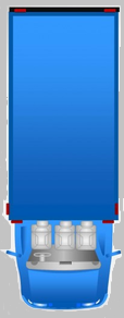
This example demonstrates acceleration changes in traffic. It involves core math concepts such as function graphs and derivatives. Using GeoGebra commands like Sequence and Segment, a dynamic traffic scenario is constructed. Suitable for high school and above students learning calculus and function graphs.
GeoGebra Commands & Parameters
Sequence((n, f(n)), n, 0, t_1) → markers_1Sequence((n, g(n)), n, 0, t_1) → markers_2Segment((-1.9, 0), (-1.1, 0)) → line_0Sequence(i - 0.4 < x < i + 0.4, i, 0, t_1) → photo_{road}Sequence(x = i - 0.4, i, 0, t_1) → left_{road}Sequence(x = i + 0.4, i, 0, t_1) → right_{road}Sequence(x = i, i, 0, t_1) → mid_{road}Sequence(Translate[truck_p, Vector[(0, f(0)), (i, f(i))]], i, 0, t_1) → photo_bSegment((-1.9, 200), (-1.1, 200)) → line_{200}Sequence(Translate[redcar_p, Vector[(0, g(0)), (i - g_y(i), g(i))]], i, 0, t_1) → photo_rSequence((i - 0.2, 100), i, 5, t_1) → crashphoto
AI Drawing Prompt Reference
Draw a traffic scenario showing changes in vehicle acceleration. Draw two parallel lines to represent the road, with vehicles and a truck on them. The truck's acceleration curve is f(t) and the vehicle's acceleration curve is g(t). From t=0 to t=t_1, both the vehicle and the truck start accelerating from rest. The vehicle collides with the truck at t=t_1.
The prompt above was compiled from the original drawing commands and is for reference only.