
The definite integral as the limit of a Riemann sum
Loading the math board and drawing, please wait…
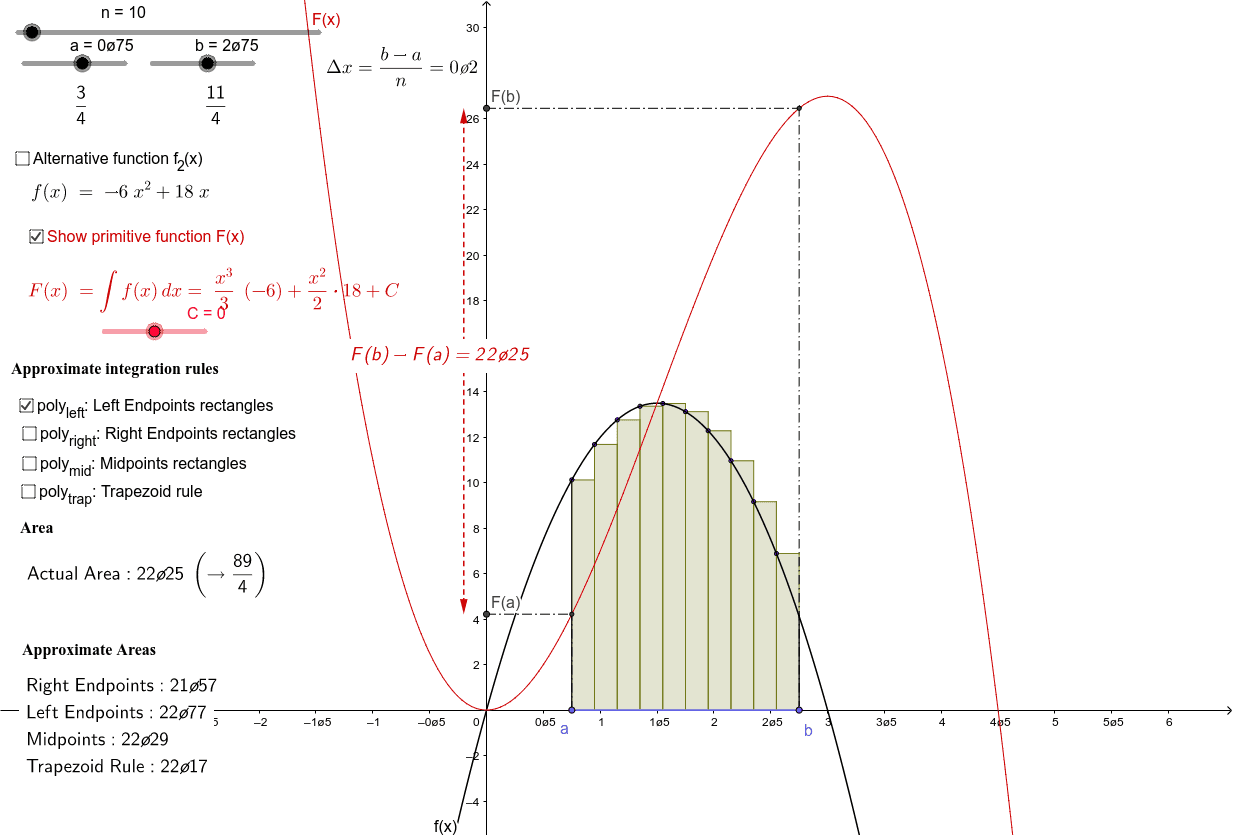
This example demonstrates how the definite integral can be calculated as the limit of a Riemann sum, visually illustrating the relationship between integration and area. Core mathematical concepts include definite integral, Riemann sum, trapezoidal rule, and vectors. GeoGebra commands and objects like If, Sequence, Integral, LaTeX, Segment, FractionText, Midpoint, Vector, Distance, Intersect, and Point are used to construct the animation showing the integration process. Suitable for high school and above students to learn and understand basic calculus concepts.
GeoGebra Commands & Parameters
If(f_{alt}, f_2, f) → f_1Sequence(a + (i * (b - a) / n), i, 0, n) → x_iIntegral(f_1, a, b) → S_{actual}Sequence((1 / 2 * (a + (i * (b - a) / n) + a + ((i + 1) * (b - a) / n))), i, 0, n) → midSequence(f_1((1 / 2 * (a + (i * (b - a) / n) + a + ((i + 1) * (b - a) / n)))), i, 0, n - 1) → functionvaluesmidSequence(Polygon[(Element[x_i, i], 0), (Element[x_i, i + 1], 0), (Element[x_i, i + 1], Element[functionvaluesmid, i]), (Element[x_i, i], Element[functionvaluesmid, i])], i, 1, n) → poly_{mid}Sequence(f_1((p_1 * (a + (i * (b - a) / n))) + ((1 - p_1) * (a + ((i + 1) * (b - a) / n)))), i, 0, n - 1) → functionvaluespSequence(Polygon[(Element[x_i, i], 0), (Element[x_i, i + 1], 0), (Element[x_i, i + 1], Element[functionvaluesp, i]), (Element[x_i, i], Element[functionvaluesp, i])], i, 1, n) → poly4LaTeX("Midpoints: " + S_{mid}) → text4Sequence((Element[mid, i], Element[functionvaluesmid, i]), i, 1, n) → pointsmidSequence(((p_1 * (a + (i * (b - a) / n))) + ((1 - p_1) * (a + ((i + 1) * (b - a) / n))), f_1((p_1 * (a + (i * (b - a) / n))) + ((1 - p_1) * (a + ((i + 1) * (b - a) / n))))), i, 0, n - 1) → pointspLaTeX("p=" + p_1 + ",\;(1-p)=" + (1 - p_1) + "\;Center\;Points:" + S_p) → text5Segment(A_1, B_2) → lLaTeX("f(x)\;=\;" + f_1) → text9Sequence(Polygon[(Element[x_i, i], 0), (Element[x_i, i + 1], 0), (Element[x_i, i + 1], Element[y_i, i]), (Element[x_i, i], Element[y_i, i])], i, 1, n) → poly_{left}FractionText(b) → text_bFractionText(a) → text_aSequence((Element[x_i, i], Element[y_i, i]), i, 1, n) → pointsleftSequence((Element[x_i, i + 1], Element[y_i, i + 1]), i, 1, n) → pointsrightSequence(Polygon[(Element[x_i, i], 0), (Element[x_i, i + 1], 0), (Element[x_i, i + 1], Element[y_i, i + 1]), (Element[x_i, i], Element[y_i, i + 1])], i, 1, n) → poly_{right}Sequence(Polygon[(Element[x_i, i], 0), (Element[x_i, i + 1], 0), (Element[x_i, i + 1], Element[y_i, i + 1]), (Element[x_i, i], Element[y_i, i])], i, 1, n) → poly_{trap}Sequence((Element[x_i, i], Element[y_i, i]), i, 1, n + 1) → pointstrapLaTeX("Right\;Endpoints: " + S_{right}) → text1_1LaTeX("Left\;Endpoints: " + S_{left}) → text3Midpoint(H, J) → EVector(E, J) → uVector(E, H) → vDistance(H, J) → distanceHJIntersect(F, r, (2.75, 26.46875)) → GIntersect(F, s, (0.75, 4.21875)) → ISegment(B_2, G) → mPoint(poly_{left}) → KSegment(K, I) → tIntegral(f_1) → F_0LaTeX("F(x)\;=\int f(x) \, dx=\;" + F_0 + " + C") → text_FSegment(D, G) → a_1Segment(C_1, I) → b_1Intersect(f_1, s, (0.75, 10.125)) → AIntersect(f_1, r, (2.75, 4.125)) → BSegment(A, A_1) → hSegment(B, B_2) → jLaTeX("Trapezoid\;Rule: " + S_{trap}) → text6