
Convergence of Improper Integrals of Power Functions
Loading the math board and drawing, please wait…
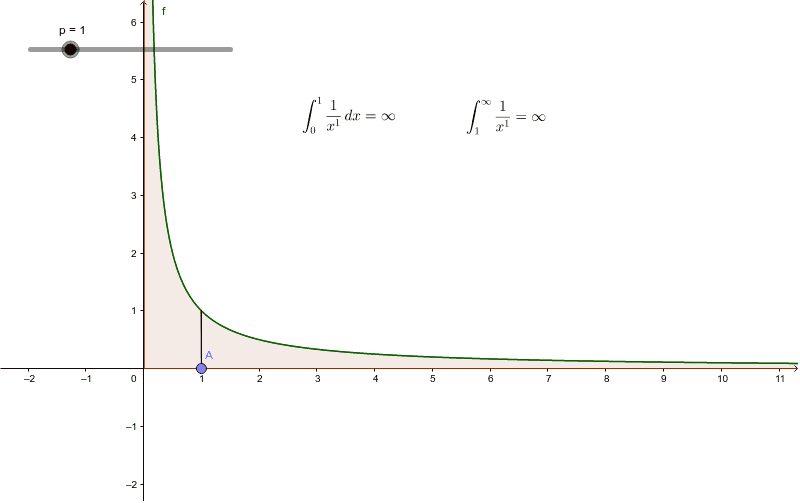
This example demonstrates the graphical behavior of the convergence of improper integrals of power functions as the exponent changes. Key math concepts include improper integrals, convergence, power function properties, and limits. GeoGebra commands used in construction are Point, OrthogonalLine, Intersect, Segment, and Integral. Suitable for high school and above mathematics learners to visually understand the convergence conditions of power function integrals.
GeoGebra Commands & Parameters
Point(xAxis) → AOrthogonalLine(A, xAxis) → aIntersect(f, a, (1, 1)) → BSegment(A, B) → bIntegral(f, 0.01, x(A)) → cIntegral(f, x(A), 1000) → d
AI Drawing Prompt Reference
Draw an x-axis and a line perpendicular to it, meeting at point P. Find point Q on function f such that line PQ intersects at (1,1). Connect P and Q with line segment R. Calculate and shade the integral areas of function f from 0.01 to x(P) and from x(P) to 1000.
The prompt above was compiled from the original drawing commands and is for reference only.