
Taylor Series Expansion Demo
Loading the math board and drawing, please wait…
This example demonstrates the Taylor series expansion of a function f(x) around x=0. It involves core mathematical concepts such as function approximation, infinite series, and properties of trigonometric functions. Key GeoGebra commands used include Point, Segment, Polygon, Text, Sequence, and Midpoint to construct function graphs, polynomial approximations, and dynamic visualizations. Suitable for high school students and math enthusiasts to understand function approximation theory and the geometric meaning of Taylor series.
GeoGebra Commands & Parameters
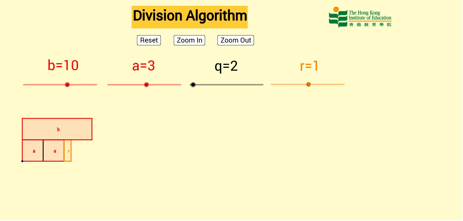
Point(Circle[A, abs((a * q))]) → BSegment(A, B) → cPolygon(A + (abs(c), 0), A + (abs(c), 6), A + (0, 6), A) → poly1, d, e, f, nPolygon(C + (abs(r), 0), C + (abs(r), 6), C + (0, 6), C) → poly2, g, h, i, pPolygon(D + (abs(b), 0), D + (abs(b), 6), D + (0, 6), D) → poly3, j, k, l, mText(("a=" * a)) → text3Text(("b=" * b)) → text4Text(("q=" * q)) → text5Text(("r=" * r)) → text6Text("b", D + (abs(b) / 2, 2.4)) → text1Sequence(Text["a", A + (abs(a) / 2 + (abs(a) * p), 2.4)], p, 0, q - 1) → list2Sequence(Segment[A + ((i * abs(a)), 0), A + ((i * abs(a)), 6)], i, 1, q) → list1Text("r", A + ((q * abs(a)) + abs(r) / 2, 2.4)) → text2Midpoint(Midpoint[Corner[4], Midpoint[Corner[4], Midpoint[Corner[4], Corner[1]]]], Midpoint[Corner[4], Midpoint[Corner[4], Corner[1]]]) → OMidpoint(Midpoint[Corner[3], Midpoint[Corner[3], Midpoint[Corner[3], Corner[2]]]], Midpoint[Corner[3], Midpoint[Corner[3], Corner[2]]]) → P